The beginner’s guide to implementing YOLOv3 in TensorFlow 2.0 (part-1)

Tutorial Overview

What is this post about?

Over the past few years in Machine learning, we’ve seen dramatic progress in the field of object detection. Although there are several different models of object detection, in this post, we’re going to discuss specifically one model called “You Only Look Once” or in short YOLO.

Invented by Joseph Redmon, Santosh Divvala, Ross Girshick and Ali Farhadi (2015), YOLO has already 3 different versions so far. But in this post, we’are going to focus on the latest version only, that is YOLOv3. So here, you’ll be discovering how to implement the YOLOv3 algorithm in TensorFlow 2.0 in the simplest way.

For more details about how to install TensorFlow 2.0, you can follow my previous tutorial here.

Who is this tutorial for?

When I got started learning YOLO a few years ago, I found that it was really difficult for me to understand both the concept and implementation. Even though there are tons of blog posts and GitHub repos about it, most of them are presented in complex architectures.

I pushed myself to learn them one after another and it ended me up to debug every single code, step by step, in order to grasp the core of the YOLO concept. Fortunately, I didn’t give up. After spending a lot of time, I finally made it works.

Based on that experience, I tried to make this tutorial easy and useful for many beginners who just got started learning object detection. Without over-complicating things, this tutorial can be a simple explanation of YOLOv3’s implementation in TensorFlow 2.0.

Prerequisites

• Familiar with Python 3
• Understand object detection and Convolutional Neural Networks (CNNs).
• Basic TensorFlow usage.

What will you get after completing this tutorial?

After completing this tutorial, you will understand the principle of YOLOv3 and know how to implement it in TensorFlow 2.0. I believe this tutorial will be useful for a beginner who just got started learning object detection.

This tutorial is broken into 4 parts, they are:

1. Part-1, An introduction of the YOLOv3 algorithm.
2. Part-2, Parsing the YOLOv3 configuration file and creating the YOLOv3 network.
3. Part-3, Converting the YOLOv3 pre-trained weights into the TensorFlow 2.0 weights format.
4. Part-4, Encoding bounding boxes and testing this implementation with images and videos.

Now, it’s time to get started on this tutorial with a brief overview of everything that we’ll be seeing in this post.

YOLO: YOLOv3

Initially, for those of you who don’t have a lot of prior experience with this topic, I’m going to do a brief introduction about YOLOv3 and how the algorithm actually works.

As its name suggests, YOLO – You Only Look Once, it applies a single forward pass neural network to the whole image and predicts the bounding boxes and their class probabilities as well. This technique makes YOLO a super-fast real-time object detection algorithm.

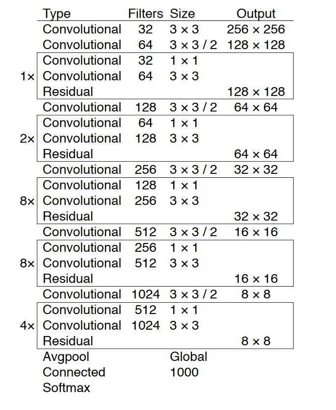
As mentioned in the original paper (the link is provided at the end of this part), YOLOv3 has 53 convolutional layers called Darknet-53 as you can see in the following figure.

How YOLOv3 works?

The YOLOv3 network divides an input image into S x S grid of cells and predicts bounding boxes as well as class probabilities for each grid. Each grid cell is responsible for predicting B bounding boxes and C class probabilities of objects whose centers fall inside the grid cell. Bounding boxes are the regions of interest (ROI) of the candidate objects. The “B” is associated with the number of using anchors. Each bounding box has (5 + C) attributes. The value of “5” is related to 5 bounding box attributes, those are center coordinates (b_x, b_y) and shape (b_h, b_w) of the bounding box, and one confidence score. The “C” is the number of classes. The confidence score reflects how confidence a box contains an object. The confidence score is in the range of 0 – 1. We’ll be talking this confidence score in more detail in the section Non-Maximum Suppression (NMS).

Since we have S x S grid of cells, after running a single forward pass convolutional neural network to the whole image, YOLOv3 produces a 3-D tensor with the shape of [S, S, B * (5 + C].

The following figure illustrates the basic principle of YOLOv3 where the input image is divided into the 13 x 13 grid of cells (13 x 13 grid of cells is used for the first scale, whereas YOLOv3 actually uses 3 different scales and we're going to discuss it in the section prediction across scale).

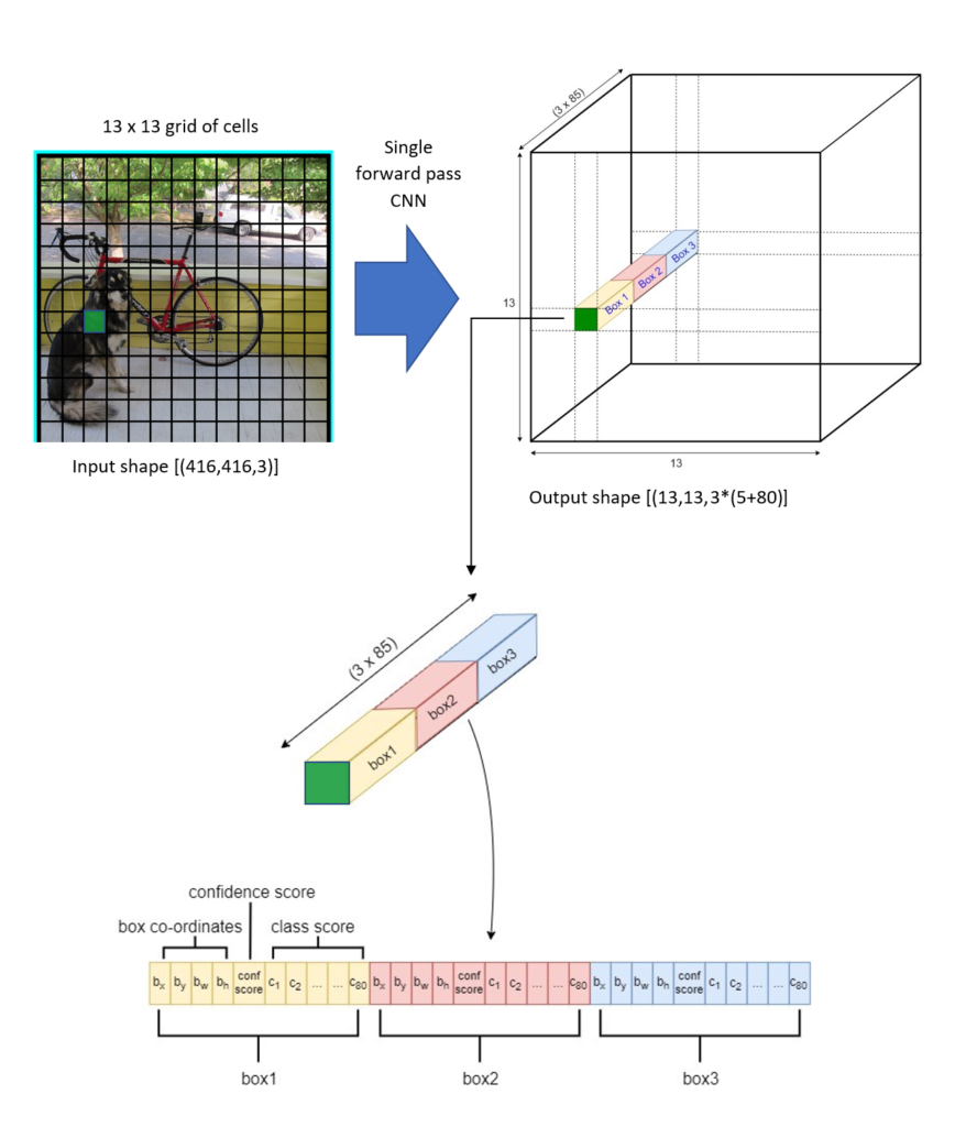
YOLOv3 was trained on the COCO dataset with C=80 and B=3. So, for the first prediction scale, after a single forward pass of CNN, the YOLOv3 outputs a tensor with the shape of [(13, 13, 3 * (5 + 80)].

Anchor Box Algorithm

Basically, one grid cell can detect only one object whose mid-point of the object falls inside the cell, but what about if a grid cell contains more than one mid-point of the objects?. That means there are multiple objects overlapping. In order to overcome this condition, YOLOv3 uses 3 different anchor boxes for every detection scale.

The anchor boxes are a set of pre-defined bounding boxes of a certain height and width that are used to capture the scale and different aspect ratio of specific object classes that we want to detect.

While there are 3 predictions across scale, so the total anchor boxes are 9, they are: (10×13), (16×30), (33×23) for the first scale, (30×61), (62×45), (59×119) for the second scale, and (116×90), (156×198), (373×326) for the third scale.

A clear explanation of the anchor box’s concept can be found in Andrew NG’s video here.

Prediction Across Scale

YOLOv3 makes detection in 3 different scales in order to accommodate different objects size by using strides of 32, 16 and 8. This means, if we feed an input image of size 416 x 416, YOLOv3 will make detection on the scale of 13 x 13, 26 x 26, and 52 x 52.

For the first scale, YOLOv3 downsamples the input image into 13 x 13 and makes a prediction at the 82nd layer. The 1st detection scale yields a 3-D tensor of size 13 x 13 x 255.

After that, YOLOv3 takes the feature map from layer 79 and applies one convolutional layer before upsampling it by a factor of 2 to have a size of 26 x 26. This upsampled feature map is then concatenated with the feature map from layer 61. The concatenated feature map is then subjected to a few more convolutional layers until the 2nd detection scale is performed at layer 94. The second prediction scale produces a 3-D tensor of size 26 x 26 x 255.

The same design is again performed one more time to predict the 3rd scale. The feature map from layer 91 is added one convolutional layer and is then concatenated with a feature map from layer 36. The final prediction layer is done at layer 106 yielding a 3-D tensor of size 52 x 52 x 255.

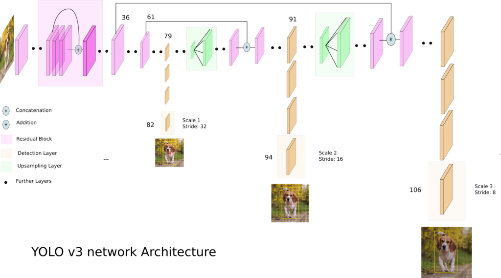
Once again, YOLOv3 predicts over 3 different scales detection, so if we feed an image of size 416x 416, it produces 3 different output shape tensor, 13 x 13 x 255, 26 x 26 x 255, and 52 x 52 x 255.

Bounding box Prediction

For each bounding box, YOLO predicts 4 coordinates, t_x, t_y, t_w, t_h. The t_x and t_y are the bounding box’s center coordinate relative to the grid cell whose center falls inside, and the t_w and t_h are the bounding box’s shape, width and height, respectively.

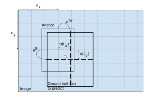
The final output of the bounding box predictions need to be refined based on this formula:

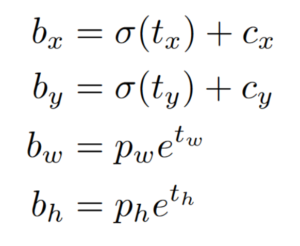
The p_w and p_h are the anchor’s width and height, respectively. The figure below describes this transformation in more detail.

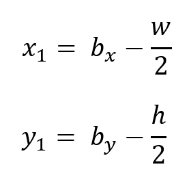
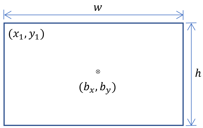
The YOLO algorithm returns bounding boxes in the form of (b_x, b_y, b_w, b_h). The b_x and b_y are the center coordinates of the boxes and b_w and b_h are the box shape (width and height). Generally, to draw boxes, we use the top-left coordinate (x₁, y₁) and the box shape (width and height). To do this just simply convert them using this simple relation:

Total Class Prediction

Using the COCO dataset, YOLOv3 predicts 80 different classes. YOLO outputs bounding boxes and class prediction as well. If we split an image into a 13 x 13 grid of cells and use 3 anchors box, the total output prediction is 13 x 13 x 3 or 169 x 3. However, YOLOv3 uses 3 different prediction scales which splits an image into (13 x 13), (26 x 26) and (52 x 52) grid of cells and with 3 anchors for each scale. So, the total output prediction will be ([(13 x13) + (26×26)+(52×52)] x3) =10,647.

Non-Maximum Suppression

Actually, after single forward pass CNN, what’s going to happen is the YOLO network is trying to suggest multiple bounding boxes for the same detected object. The problem is how do we decide which one of these bounding boxes is the right one.

Fortunately, to overcome this problem, a method called non-maximum suppression (NMS) can be applied. Basically, what NMS does is to clean up these detections. The first step of NMS is to suppress all the predictions boxes where the confidence score is under a certain threshold value. Let’s say the confidence threshold is set to 0.5, so every bounding box where the confidence score is less than or equal to 0.5 will be discarded.

Yet, this method is still not sufficient to choose the proper bounding boxes, because not all unnecessary bounding boxes can be eliminated by this step, so then the second step of NMS is applied. The rest of the higher confidence scores are sorted from the highest to the lowest one, then highlight the bounding box with the highest score as the proper bounding box, and after that find all the other bounding boxes that have a high IOU (intersection over union) with this highlighted box. Let’s say we’ve set the IOU threshold to 0.5, so every bounding box that has IOU greater than 0.5 must be removed because it has a high IOU that corresponds to the same highlighted object. This method allows us to output only one proper bounding box for a detected object. Repeat this process for the remaining bounding boxes and always highlight the highest score as an appropriate bounding box. Do the same step until all bounding boxes are selected properly.

I have another tutorial that I highly recommend reading. It provides detailed instructions on how to load and visualize the COCO dataset using custom code.

End Notes

Here’s a brief summary of what we have covered in this part:

• YOLO applies a single neural network to the whole image and predicts the bounding boxes and class probabilities as well. This makes YOLO a super-fast real-time object detection algorithm.
• YOLO divides an image into SxS grid cells. Every cell is responsible for detecting an object whose center falls inside.
• To overcome the overlapping objects whose centers fall in the same grid cell, YOLOv3 uses anchor boxes.
• To facilitate the prediction across scale, YOLOv3 uses three different numbers of grid cell sizes (13×13), (26×26), and (52×52).
• A Non-Max Suppression is used to eliminate the overlapping boxes and keep only the accurate one.

If I missed something or you have any questions, please don’t hesitate to let me know in the comments section.

After a brief introduction, now it’s time for us to jump into the technical details. So, let’s go get part-2.

Parts

• Part-1, An introduction of the YOLOv3 algorithm
• Part-2, Parsing the YOLOv3 configuration file and creating the YOLOv3 network
• Part-3, Converting the YOLOv3 pre-trained weights into the TensorFlow 2.0 weights format
• Part-4, Encoding bounding boxes and testing this implementation with images and videos

Links to the original YOLO’s papers:

• v1, You Only Look Once: Unified, Real-Time Object Detection https://arxiv.org/pdf/1506.02640.pdf
• v2, YOLO9000: Better, Faster, Stronger https://arxiv.org/pdf/1612.08242.pdf
• v3, YOLOv3: An Incremental Improvement https://pjreddie.com/media/files/papers/YOLOv3.pdf

Recently Posted Tutorials

• COCO Dataset: A Step-by-Step Guide to Loading and Visualizing with Custom Code
• A Comprehensive Guide to Gradient Descent Algorithm
• How to Create a Custom Dataset Class in PyTorch