Guide to Gradient Descent Algorithm: A Comprehensive implementation in Python

Posted by Rahmad Sadli on January 7, 2023 in Deep Learning, Machine Learning, Object Classification, Object Detection, Python Programming

Gradient Descent Python
gradient descent from scratch python

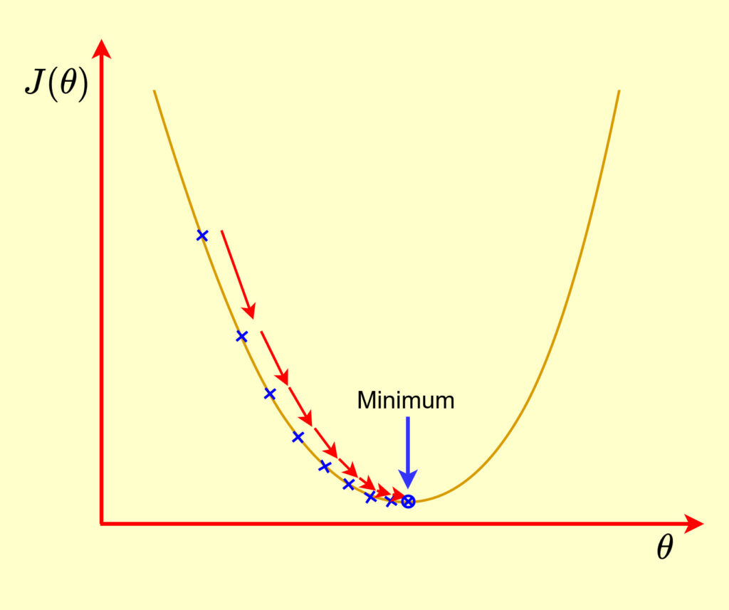
Let’s learn about one of important topics in the field of Machine learning, a very-well-known algorithm, Gradient descent. Gradient descent is a widely-used optimization algorithm that optimizes the parameters of a Machine learning model by minimizing the cost function. Gradient descent updates the parameters iteratively during the learning process by calculating the gradient of the cost function with respect to the parameters.

The parameters are updated in the opposite direction of the gradient of the cost function, which means that if the gradient is positive, the parameters will be decreased and vice versa in order to reduce the cost. In other words, Gradient descent updates the parameters in the direction that reduces the cost function. This process is done repeatedly until the smallest cost function is achieved.

If you want to understand better about how this algorithm is developed from math equations to code implementation, you are in the right place because in this tutorial, we will discuss this algorithm in more detail.

Before we get started, it is important to mention that the algorithm you will be learning today is one of the fundamental topics in the field of Machine learning. A strong foundation in calculus and algebra is highly recommended for better understanding this algorithm. Having said that, I’ll do my best to explain as good as I can in order to make you understand better about this topic. You can also help yourself by learning the calculus and algebra if you think it’s necessary for you to understand this topic.

There are several types of Gradient descent, including batch-Gradient descent, stochastic Gradient descent (SGD), and mini-batch Gradient descent. Each type has its own trade-offs in terms of computational efficiency and the accuracy of updating the parameters. However, in today’s tutorial, we’ll be focusing only on the vanila Gradient descent or better known as batch Gradient descent. We will cover the other types in the next tutorials.

Ok, without further ado, here is the outline for today’s tutorial:

Linear Regression
Gradient Descent
Python Implementation
Conclusion
References

Before we get started learning Gradient descent, I will introduce you to Linear regression first, because they are closely related. Gradient descent is often used as an optimization algorithm to find the optimal solution for the parameters in a Linear regression model. By understanding how gradient descent works and how it can be used to solve linear regression problems, you can gain a deeper understanding of Gradient descent and how it can be applied in machine learning and other areas.

So, we’ll start off this tutorial by learning Linear regression first and after that we’ll continue with Gradient descent and Python implementation.

Linear regression

What is Linear regression?

Linear regression is a supervised algorithm that draws a linear relationship model between the independent variables (inputs, sometimes it is called regressors or predictors) and the dependent variable (output or outcome). In simple words, the idea of Linear regression is to find the line that fits the observed data and use it to predict the future outcome from new inputs or unseen data. The observed data can be a historical data that has been collected for a specific purpose within a certain duration.

Linear regression is widely used in financial and business analysis fields including to predict stocks and commodity prices, sales forecasting, employee performance analysis, etc.

The simple Linear regression consists of only one independent variable ( $x$ ) and one dependent variable ( $y$ ) as illustrated in the following figure. What we actually do in Linear regression is basically to find the best parameters that fits the straight line to the observations by minimizing the errors between the predicted outcomes and the observations. Meaning that, the best model in Linear regression is the linear equation model with the best parameters.

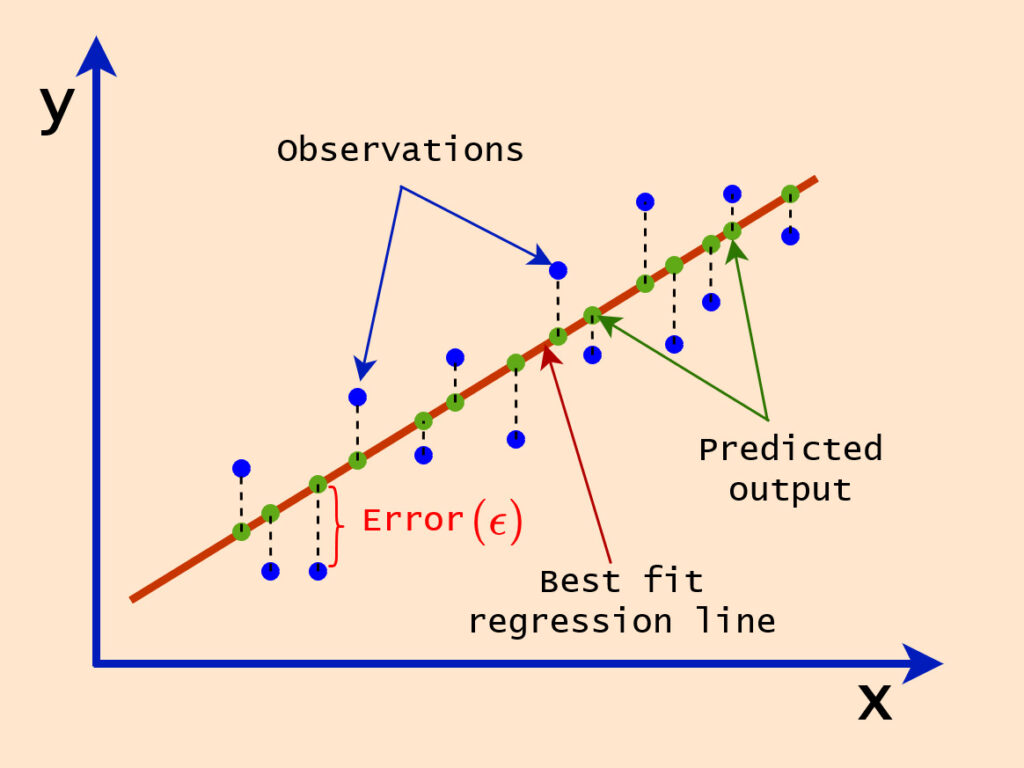
The figure above describes the simple Linear regression problem. The red line is called the regression line, which is the line that best fits the given observations that can be used to predict the unseen inputs.

Now, you already know what the regression problem is, which is the problem of how to obtain the best parameters in order to have the stright line representing the best relationship between the input and the outcome. Cool! so now let’s look at the following figure.

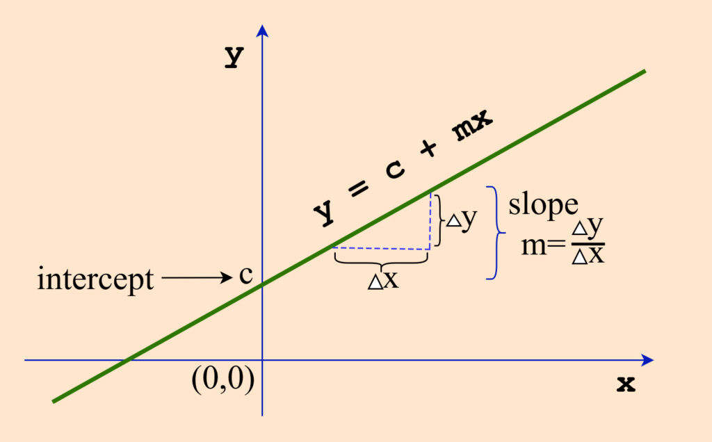
I’m pretty sure that you are very familiar with this figure. Yup, It is the figure of line equation model of $y= mx +c$ , where $m$ represents the slope or gradient or rate of change ( $\frac{\Delta y}{\Delta x}$ ), and $c$ is the $y$ -intercept.

Simple Linear Regression Hypothesis

A Linear regression line has the similiar equation to the line equation mentioned above. However, to describe the relationship between variables, in Linear regression we commonly use different notations. A simple Linear regression with one independent variable and one dependent variable is defined as:

(1) $\begin{equation*}\boxed{h_{\bm{\theta}} (\text{x}) = \theta_0 +\theta_1\text{x}}\end{equation*}$

where $h_{\bm{\theta}} (\text{x})$ is the hypothesis function, $\text{x}$ is the input, and $\theta_0$ and $\theta_1$ are the parameters of the model. The subscript $\theta$ means that the hypothesis depends not only on the input $\text{x}$ but also on the parameters $\theta_0$ and $\theta_1$ .

Here, we can see the regression hypthotesis is exactly the same as the line equation. However, in Linear regression, we use different notations as already mentioned. We use $\theta_0$ and $\theta_1$ to represent the $y$ -intercept and the slope, respectively.

We use the notation $h_{\bm{\theta}} (\text{x})$ for the output/prediction is because what we actually do in Linear regression is that we’re trying to estimate the output from the estimated parameters and the given inputs. Each time we’re trying to fit the model to the observed data, we always chose/estimate new parameters. And after that, we use the hypothesis to validate whether the chosen parameters are better fits with the observations or not by calculating the errors between the hypothesis and the observations.

Multi-variable Linear Regression

In Linear regression, we usually have one dependent variable as a target output. The inputs, however, can consist of one or more independent variables. We’ve just looked at a simple Linear regression with only one input variable. Now, we’re going to look at multi-variable Linear regression.

Let $\text{x}$ be a row vector of an input where $\text{x} \in \mathbb{R}^{n+1}$ and $\bm{\theta}$ be a column vector of parameters, where $\bm{\theta} \in \mathbb{R}^{n+1}$ . So that $\text{x}$ and $\bm{\theta}$ can be written as follows:

(2) $\begin{equation*}\text{x} =\begin{bmatrix}x_0 & x_1 & x_2 & x_3 & ... & x_n\\\end{bmatrix}\in \mathbb{R}^{n+1}\text{, and }\bm{\theta} =\begin{bmatrix}\theta_0 \\\theta_1 \\\theta_2 \\\theta_3 \\\vdots \\\theta_n \\\end{bmatrix}\in \mathbb{R}^{n+1}\end{equation*}$

SHORT NOTICE!
Now, the input $\text{x}$ contain $n+1$ variables, $x_0,x_1,x_2,...,x_n$ . These variables are called as features. So, $\text{x}$ contains $n+1$ $features$ .

Then the hypothesis of Linear regression given $\text{x}$ and $\bm{\theta}$ can be written as follows:

(3) $\begin{equation*}\boxed{h_{\bm{\theta}} (\text{x}) = \theta_0 +x_1\theta_1+ x_2\theta_2+…+x_n\theta_n\qquad\qquad\qquad\text{, where:}\ x_0=1}\end{equation*}$

We can rewrite this relation in the following form:

(4) $\begin{equation*}\boxed{h_{\bm{\theta}} (\text{x}) = \sum_{j=0}^n x_j\theta_j\qquad\qquad\qquad\text{, where:}\ x_0=1}\end{equation*}$

The equation (4) can be written in a dot product of two matrices form as follows:

(5) $\begin{equation*}h_{\bm{\theta}} (\text{x}) = \underbrace{\begin{bmatrix}x_0 & x_1 & x_2 & x_3 & ... & x_n\end{bmatrix}}_{\text{x}}\underbrace{\begin{bmatrix}\theta_0 \\\theta_1 \\\theta_2 \\\theta_3 \\\vdots \\\theta_n \\\end{bmatrix}}_{\bm{\theta}}\qquad\qquad\qquad\text{, where:}\ x_0=1\end{equation*}$

So, the hypothesis of Linear regression can be written it in a vectorized form as follows:

(6) $\begin{equation*}\boxed{ \textcolor{blue} {h_{\bm{\theta}} (\text{x}) = \text{x}\bm{\theta}}}\end{equation*}$

IMPORTANT!
You must be very carefull when arranging your data. For example, if you arrange both $\text{x}$ and $\bm{\theta}$ as column vectors as follows:

(7) $\begin{equation*}\text{x} =\begin{bmatrix}x_0 \\x_1\\x_2 \\ x_3 \\\vdots\\ x_n\end{bmatrix}\in \mathbb{R}^{n+1}\text{, and }\bm{\theta} =\begin{bmatrix}\theta_0 \\\theta_1 \\\theta_2 \\\theta_3 \\\vdots \\\theta_n \\\end{bmatrix}\in \mathbb{R}^{n+1}\end{equation*}$

Then, one of them must be transposed, either $\text{x}$ or $\bm{\theta}$ . Otherwise, you will get an error when you perform a dot product. Therefore, in this case, the hypothesis can be written as:

(8) $\begin{equation*}\boxed{h_{\bm{\theta}} (\text{x}) = \text{x}^T\bm{\theta}\qquad\qquad\qquad\text{, where:}\ x_0=1}\end{equation*}$

(9) $\begin{equation*}\boxed{h_{\bm{\theta}} (\text{x}) = \bm{\theta}^T\text{x}\qquad\qquad\qquad\text{, where:}\ x_0=1}\end{equation*}$

NOTICE!
To avoid confusion, I will consistently use a format for input data $\text{x}$ where its columns represent features, and for $\bm{\theta}$ I’ll keep it as a column vector as in (2).

After we have the hypothesis function, what we need to do now is to find the best parameters for this hypothesis, so that we can have the best model to predict our new input. To do so, we’re going to use Gradient descent algorithm.

I hope you’re ready now to learn the Gradient descent. Ok. Let’s go!

Gradient Descent

What is Gradient Descent?

Gradient descent is an optimization algorithm that is commonly used in machine learning to learn a model by focusing on minimizing the cost function $J(\bm{\theta})$ w.r.t the parameters $\bm{\theta}$ . The cost function is nothing but the error between the hypothesis $h_{\bm{\theta}} (\text{x})$ and the observed data $\text{y}$ .

During the learning process, we iteratively calculate the gradient of the cost function and update the parameters of the model. The parameters are updated in the opposite direction of the gradient of $J(\bm{\theta})$ . This means that if the gradient of $J(\bm{\theta})$ is positive, the parameters should be decreased and vice versa. The model continues tweaking the parameters until having the smallest possible of error $J(\bm{\theta})$ .

In more detail, if the gradient of the cost function is positive, increasing the value of the parameters will increase the cost. Therefore, to minimize the cost, the parameters should be decreased. On the other hand, if the gradient of the cost function is negative, decreasing the value of the parameters will increase the cost. In this case, the parameters should be decrease in order to minimize the cost.

Problem Formulation

What we do basically in Gradient descent is to update the parameters by minimizing the cost function $J(\theta)$ . We iterate the updating process until we have the smallest error possible. To do so, we need to define our cost function first. So in this tutorial we define our cost function $J(\theta)$ as a half-Mean Square Errors ( $\frac{1}{2}MSE$ ) between the hypothesis and the observations.

For $m$ number of training set $\{(\text{x}^{(i)}},\text{y}^{(i)}) ; i=1,2,..,m\}$ , where $\text{x} \in \mathbb{R}^{m \text{x}(n+1)}$ , $\text{y} \in \mathbb{R}^{m+1}}$ , and $\bm{\theta} \in \mathbb{R}^{n+1}$ , the cost function $J(\theta)$ can be written as follows:

(10) $\begin{equation*}\boxed{J(\bm{\theta}) = \frac{1}{2m} \sum_{i=1}^m \Bigl( h_{\bm{\theta}}(\text{x}^{(i)})-\text{y}^{(i)} \Bigl)^2}\end{equation*}$

If we just want to consider for only one training example $(\text{x},y)$ , m=1, that makes $\text{x} \in \mathbb{R}^{n+1}$ , $\bm{\theta} \in \mathbb{R}^{n+1}$ , and $y \in \mathbb{R}}$ , the cost function $J(\theta)$ can be written as:

(11) $\begin{equation*}\boxed{J(\bm{\theta}) = \frac{1}{2} \Bigl( h_{\bm{\theta}}(\text{x})-y \Bigl)^2}\end{equation*}$

From (10) and (11) you can see why we multiply the MSE by $\frac{1}{2}$ , that is because we want to cancel out the factor of $2$ when we do the derivative.

What is Gradient?

When we are talking about the Gradient descent, we need to know first about what the gradient is. Actually, the gradient of a function $f$ , denoted as $\nabla{f}$ , is nothing but a vector of its partial derivative. Gradient of a multi-variable function $f (\theta_0, \theta_1, \theta_2, ....., \theta_n )$ is writen as in the following form:

(12) $\begin{equation*}\nabla{f} &= \begin{bmatrix}\frac{\partial f} {\partial \theta_0} \vspace{.4em}\\\frac{\partial f} {\partial \theta_1} \vspace{.4em}\\\frac{\partial f} {\partial \theta_2} \vspace{.4em}\\\vdots \\\frac{\partial f} {\partial \theta_n} \vspace{.4em}\\\end{bmatrix} \end{equation*}$

Where $\partial$ is the partial derivative operator that differenciates a function with respect to one variable and treats the others as constants.

So, the gradient of $J(\bm{\theta)}$ can be written as $\nabla{J(\bm{\theta})}$ .

Now, let’s derive the Gradient descent from our cost function.

Parameters Update Rule

We already know that the parameters will be updated iteratively in the opposite direction of $\nabla{J(\bm{\theta})}$ during the learning process. Therefore, we can define the update rule for the parameters as the following:

(13) $\begin{equation*}\boxed{\bm{\theta} := \bm{\theta} - \alpha \nabla{J(\bm{\theta})}}\end{equation*}$

Where $\alpha$ is the $\text{learning rate}$ that defines how far to go for each step. $\alpha$ can range from $0$ to $1$ $( 0 <\alpha<1)$ .

If we let $\bm{\theta}}$ be a column vector and $\bm{\theta}}\in \mathbb{R}^{n+1}$ , based on (12) we can rewrite (13) as follows:

(14) $\begin{equation*}\begin{split}\begin{bmatrix}\theta_0 \\\theta_1 \\\theta_2 \\\theta_3 \\\vdots \\\theta_n \\\end{bmatrix}:= \begin{bmatrix}\theta_0 \\\theta_1 \\\theta_2 \\\theta_3 \\\vdots \\\theta_n \\\end{bmatrix}- \alpha \begin{bmatrix}\frac{\partial} {\partial \theta_0} J(\bm{\theta})\vspace{.4em}\\\frac{\partial} {\partial \theta_1} J(\bm{\theta})\vspace{.4em}\\\frac{\partial} {\partial \theta_2} J(\bm{\theta})\vspace{.4em}\\\vdots \\\frac{\partial} {\partial \theta_n} J(\bm{\theta})\vspace{.4em}\\\end{bmatrix}\end{split}\end{equation*}$

To simplify, we rewrite (14) in the following form with a notice that all the parameters must be updated simultaneously:

(15) $\begin{equation*}\boxed{\textcolor{blue} {\theta_j := \theta_j - \alpha \frac{\partial}{\partial\theta_j}J(\bm{\theta})\qquad\qquad\qquad\ \forall j \in [0,1, 2, ... , n]}}}\end{equation*}$

Gradient Descent for a Single Training Example

Great! Now I will show you how to calculate the partial derivative of $J(\bm{\theta})$ . Let’s do it first on a single training example.

Let’s rewrite again here the cost function $J(\bm{\theta})$ for a single training example $(\text{x},y)$ , where $\text{x} \in \mathbb{R}^{n+1}$ , $y \in \mathbb{R}}$ , and $\bm{\theta} \in \mathbb{R}^{n+1}$ :

(16) $\begin{equation*}\boxed{J(\bm{\theta}) = \frac{1}{2} \Bigl( h_{\bm{\theta}}(\text{x})-\text{y} \Bigl)^2 \qquad\qquad\qquad, \forall j \in [0,1, 2, ... , n]}\end{equation*}$

Substitute (16) in (15) we have:

(17) $\begin{equation*}\boxed{\theta_j := \theta_j - \alpha . \textcolor{red} {\frac{\partial}{\partial\theta_j}}$ $\textcolor{red} {\left(\frac{1}{2} \Bigl( h_{\bm{\theta}}(\text{x})-\text{y} \Bigl)^2 \right)} \qquad\qquad\ ,\forall j \in [0,1, 2, ... , n]}}\end{equation*}$

We can solve the partial derivative part in (17) , $\textcolor{red} {\frac{\partial}{\partial\theta_j}}$ $\textcolor{red} {\left(\frac{1}{2} \Bigl( h_{\bm{\theta}}(\text{x})-\text{y} \Bigl)^2 \right)}$ as in the following way:

(18) $\begin{equation*}\boxed{\begin{split}\textcolor{red} {\frac{\partial}{\partial\theta_j} \left(\frac{1}{2} \Bigl( h_{\bm{\theta}}(\text{x})-\text{y} \Bigl)^2 \right)} &= (\bcancel{2})\frac{1}{\bcancel{2}} \Bigl( h_{\bm{\bm{\theta}}}(\text{x})-\text{y} \Bigl) \frac{\partial}{\partial\theta_j} \Bigl( h_{\bm{\theta}}(\text{x})-\text{y} \Bigl) \\&= \Bigl( h_{\bm{\theta}}(\text{x})-\text{y} \Bigl) \textcolor{magenta} {\frac{\partial}{\partial\theta_j} \Bigl( h_{\bm{\theta}}(\text{x})-\text{y} \Bigl)}\end{split}}\end{equation*}$

We still have one partial derivative to solve in (18), $\textcolor{magenta} {\frac{\partial}{\partial\theta_j} \Bigl( h_{\bm{\theta}}(\text{x})-\text{y} \Bigl)}$ . To do so, simply substitute the $h_{\bm{\theta}}(\text{x})$ from (3) in this part.

Remember, the partial derivative equation is solved by differentiating a function with respect to one variable and treating the others as constants.

So from (18), for $\forall j \in [0,1, 2, … , n]$ we have:

(19) $\begin{equation*}\boxed{\begin{split}\textcolor{red} {\frac{\partial}{\partial\theta_j} \left(\frac{1}{2} \Bigl( h_{\bm{\theta}}(\text{x})-\text{y} \Bigl)^2 \right)} &= \Bigl( h_{\bm{\theta}}(\text{x})-\text{y} \Bigl) \textcolor{magenta} {\frac{\partial}{\partial\theta_j} \Bigl( h_{\bm{\theta}}(\text{x})-\text{y} \Bigl)}\\&= \Bigl( h_{\bm{\theta}}(\text{x})-\text{y} \Bigl) \textcolor{magenta} {\frac{\partial}{\partial\theta_j} \Bigl( \left(\theta_0 +\theta_1x_1+ \theta_1x_1 +…+\theta_n x_n \right) - y\Bigl)}\\&= \Bigl( h_{\bm{\theta}}(\text{x})-\text{y} \Bigl)\textcolor{magenta} {x_j}\end{split}}\end{equation*}$

Substitute back (19) in (17), we finally have the gradient descent formula for a single training example as follows:

(20) $\begin{equation*}\boxed{ \textcolor{blue} {\theta_j := \theta_j - \alpha .\Bigl( h_{\bm{\theta}}(\text{x})-y \Bigl) x_j}} \qquad\qquad\forall j \in [0,1, 2, ... , n]}\end{equation*}$

I hope that’s not too difficult to follow. So now, we can continue deriving the Gradient descent formula for multiple training examples. Ok. let’s do it!.

Gradient Descent for Multiple Training Examples

Basically, when we develop a machine learning model, we will work with multiple training examples. Therefore, to deal with this situation, we’re ready to derive Gradient descent algorithm for multiple training examples case.

Since we are dealing with multiple training examples $\{(\text{x}^{(i)}},\text{y}^{(i)}) ; i=1,2,..,m\}$ , where $\text{x} \in \mathbb{R}^{m \text{ x }(n+1)}$ , $\text{y} \in \mathbb{R}^{m}}$ , and $\bm{\theta} \in \mathbb{R}^{n+1}$ , we rewrite the cost function $J({\bm{\theta})$ that we’ve defined in (10):

(21) $\begin{equation*}\boxed{J(\bm{\theta}) = \frac{1}{2m} \sum_{i=1}^m \Bigl( h_{\bm{\theta}}(\text{x}^{(i)})-\text{y}^{(i)} \Bigl)^2}\end{equation*}$

What we’re gonna do first is to solve for the partial derivative of $J({\bm{\theta})$ . So, let’s do it now!.

(22) $\begin{equation*}\boxed{\begin{split}\frac{\partial}{\partial\theta_j} J(\bm{\theta}) &= \frac{\partial}{\partial\theta_j} \biggl(\frac{1}{2m} \sum_{i=1}^m \Bigl( h_{\bm{\theta}}(\text{x}^{(i)})-\text{y}^{(i)} \Bigl)^2 \biggl) \\&= (2)\frac{1}{2m} \sum_{i=1}^m \Bigl( h_{\bm{\theta}}(\text{x}^{(i)})-\text{y}^{(i)} \Bigl) \textcolor{red} {\frac{\partial}{\partial\theta_j} \Bigl( h_{\bm{\theta}}(\text{x}^{(i)})-\text{y}^{(i)} \Bigl)} \\&= \frac{1}{m} \sum_{i=1}^m \Bigl( h_{\bm{\theta}}(\text{x}^{(i)})-\text{y}^{(i)} \Bigl) \textcolor{red} {\frac{\partial}{\partial\theta_j} \Bigl( h_{\bm{\theta}}(\text{x}^{(i)})-\text{y}^{(i)} \Bigl)} \\&= \frac{1}{m} \sum_{i=1}^m \Bigl(h_{\bm{\theta}}(\text{x}^{(i)})-\text{y}^{(i)} \Bigl) \textcolor{red} {x_j^{(i)}}\end{split}}\end{equation*}$

Substitute (22) in (15), then we have the mechanism for updating the parameters for multiple training examples case. Finally, the Gradient descent algorithm for multiple training examples can be written as follows:

(23) $\begin{equation*}\boxed{ \textcolor{blue} {\begin{split}\text{Repeat until} & \text{ convergence } \{ \\&\theta_j := \theta_j - \frac{\alpha}{m} \sum_{i=1}^m\Bigl( h_{\bm{\theta}}(\text{x}^{(i)})-\text{y}^{(i)} \Bigl) x_j^{(i)} \qquad\ \forall {j} \in [0, 1, 2, 3, … , n]\\\}\\ \end{split}}}\end{equation*}$

Ok, now we have the Gradient descent algorithm. Let’s write it in a vectorized form.

Gradient Descent in Vectorized Form

If we have $\text{x} \in \mathbb{R}^{m\text{ x }(n+1)}$ , $\text{y} \in \mathbb{R}^{m\text{x}1}}$ , and $\bm{\theta} \in \mathbb{R}^{(n+1)\text{x}1}$ , then $\text{x}$ , $\text{y}$ , $\bm{\theta}$ are written as follows:

(24) $\begin{equation*}\fontsize{10.0pt}{10.0pt}\selectfont\text{x} =\left[\ \begin{matrix}x_0^1 & x_1^1 & x_2^1 & x_3^1& ... & x_n^1 \vspace{.4em}\\x_0^2 & x_1^2 & x_2^2 & x_3^2& ... & x_n^2 \vspace{.4em}\\x_0^3 & x_1^3 & x_2^3 & x_3^3& ... & x_n^3 \vspace{.4em}\\\vdots & \vdots & \vdots & \vdots & \vdots & \vdots \vspace{.4em}\\x_0^m & x_1^m & x_2^m & x_3^m& ... & x_n^m \vspace{.4em}\\\end{matrix}\ \right]\text{, }\bm{\theta} =\begin{bmatrix}\theta_0 \\\theta_1 \\\theta_2 \\\theta_3 \\\vdots \\\theta_n \\\end{bmatrix} \text{, and }\text{y} =\begin{bmatrix}y^1 \\y^2 \\y^3 \\\vdots \\y^m \\\end{bmatrix}\end{equation*}$

Look at back to the parameters update formula from Gradient descent algorithm:

(25) $\begin{equation*}\boxed{\begin{split}&\theta_j := \theta_j - \frac{\alpha}{m} \sum_{i=0}^m\Bigl( h_{\bm{\theta}}(\text{x}^{(i)})-\text{y}^{(i)} \Bigl) x_j^{(i)} \qquad\ \forall {j} \in [0, 1, 2, 3, … , n]\\\end{split}}\end{equation*}$

We can write (25) in a matrix form as follows:

(26) $\begin{equation*}\begin{split}\begin{bmatrix}\theta_0 \\\theta_1 \\\theta_2 \\\theta_3 \\\vdots \\\theta_n \\\end{bmatrix}:= \begin{bmatrix}\theta_0 \\\theta_1 \\\theta_2 \\\theta_3 \\\vdots \\\theta_n \\\end{bmatrix}- \frac{\alpha}{m} \textcolor{red} {\left(}\underbrace{\underbrace{\begin{bmatrix}h_{\bm{\theta}}(\text{x}^{(1)})-\text{y}^{(1)} & h_{\bm{\theta}}(\text{x}^{(2)})-\text{y}^{(2)} & ... & h_{\bm{\theta}}(\text{x}^{(m)})-\text{y}^{(m)} \vspace{.4em}\\\end{bmatrix}}_{\text{1xm}}\underbrace{\begin{bmatrix}x_0^1 & x_1^1 & x_2^1 & ... & x_n^1 \vspace{.4em}\\x_0^2 & x_1^2 & x_2^2 & ... & x_n^2 \vspace{.4em}\\x_0^3 & x_1^3 & x_2^3 & ... & x_n^3 \vspace{.4em}\\\vdots & \vdots & \vdots & \vdots & \vdots \vspace{.4em}\\x_0^m & x_1^m & x_2^m & ... & x_n^m \vspace{.4em}\\\end{bmatrix}}_{\text{m x (n+1)}}}_{\text{Result: a matrix of size 1 x (n+1)}}\right)^T\\\end{split}\end{equation*}$

Why do we need to transpose the red part of the (26)?

The answer for this is because the dot product of these matrices is a matrix of size $\text{1 x (n+1)}$ . Since the dimension of $\bm{\theta}$ is $\text{(n+1) x 1}$ , then the transpose of the matrix is required in order to have the same matrix size. That’s it, hope you can understand.

Since we have:

(27) $\begin{equation*}\boxed{h_{\bm{\theta}} (\text{x}) = \theta_0 +x_0\theta_1+ x_1\theta_1+x_2\theta_2 +…+x_n\theta_n}\end{equation*}$

Then, the (26) can be rewritten in the following form:

(28) $\begin{equation*}\boxed{\begin{split}\begin{bmatrix}\theta_0 \\\theta_1 \\\theta_2 \\\theta_3 \\\vdots \\\theta_n \\\end{bmatrix}:= \begin{bmatrix}\theta_0 \\\theta_1 \\\theta_2 \\\theta_3 \\\vdots \\\theta_n \\\end{bmatrix}- \frac{\alpha}{m} \left(\textcolor{red} {\left[\ \begin{array}{@{}*{11}{c}@{}}(\theta_0x_0^1+\theta_1x_1^1+\theta_2x_2^1+...+\theta_nx_n^1)-y^1 \vspace{.4em}\\(\theta_0x_0^2+\theta_1x_1^2+\theta_2x_2^2+...+\theta_nx_n^2)-y^2 \vspace{.4em}\\(\theta_0x_0^3+\theta_1x_1^3+\theta_2x_2^3+…+\theta_nx_n^3)-y^3 \vspace{.4em}\\\vdots \\(\theta_0x_0^m+\theta_1x_1^m+\theta_2x_2^m+...+\theta_nx_n^2)-y^m \vspace{.4em}\\\end{array}\ \right]^T}\left[\ \begin{array}{@{}*{11}{c}@{}}x_0^1 & x_1^1 & x_2^1 & ... & x_n^1 \vspace{.4em}\\x_0^2 & x_1^2 & x_2^2 & ... & x_n^2 \vspace{.4em}\\x_0^3 & x_1^3 & x_2^3 & ... & x_n^3 \vspace{.4em}\\\vdots & \vdots & \vdots & \vdots & \vdots \vspace{.4em}\\x_0^m & x_1^m & x_2^m & ... & x_n^m \vspace{.4em}\\\end{array}\ \right]\right)^T\\\end{split}}\end{equation*}$

Then we can write (28) in the following form:

(29) $\begin{equation*}\begin{split}\underbrace{\begin{bmatrix}\theta_0 \\\theta_1 \\\theta_2 \\\theta_3 \\\vdots \\\theta_n \\\end{bmatrix}}_{\bm{\theta}}:= \underbrace{\begin{bmatrix}\theta_0 \\\theta_1 \\\theta_2 \\\theta_3 \\\vdots \\\theta_n \\\end{bmatrix}}_{\bm{\theta}}- \frac{\alpha}{m} \left(\textcolor{red} {\left(\underbrace{\begin{bmatrix}x_0^1 & x_1^1 & x_2^1 & ... & x_n^1 \vspace{.4em}\\x_0^2 & x_1^2 & x_2^2 & ... & x_n^2 \vspace{.4em}\\x_0^3 & x_1^3 & x_2^3 & ... & x_n^3 \vspace{.4em}\\\vdots & \vdots & \vdots & \vdots & \vdots \vspace{.4em}\\x_0^m & x_1^m & x_2^m & ... & x_n^m \vspace{.4em}\\\end{bmatrix}}_{\text{x}} \underbrace{\begin{bmatrix}\theta_0 \\\theta_1 \\\theta_2 \\\vdots \\\theta_n \\\end{bmatrix}}_{\bm{\theta} }- \underbrace{\begin{bmatrix}y^1 \\y^2 \\y^3 \\\vdots \\y^m \\\end{bmatrix}}_{\text{y}} \right)^T}\underbrace{\begin{bmatrix}x_0^1 & x_1^1 & x_2^1 & ... & x_n^1 \vspace{.4em}\\x_0^2 & x_1^2 & x_2^2 & ... & x_n^2 \vspace{.4em}\\x_0^3 & x_1^3 & x_2^3 & ... & x_n^3 \vspace{.4em}\\\vdots & \vdots & \vdots & \vdots & \vdots \vspace{.4em}\\x_0^m & x_1^m & x_2^m & ... & x_n^m \vspace{.4em}\\\end{bmatrix}}_{\text{x}}\right)^T\end{split}\end{equation*}$

Finally, we can write (29) in a vectorized form as follows:

(30) $\begin{equation*}\boxed{\begin{split}\bm{\theta} & := \bm{\theta} - \frac{\alpha}{m} \left(\left(\text{x}\bm{\theta}-\text{y}\right)^T\text{x}\right)^T\\& := \bm{\theta} - \frac{\alpha}{m} \left(\text{x}^T(\text{x}\bm{\theta}-\text{y})\right)\end{split}} \end{equation*}$

where $\text{x}\bm{\theta}$ is our hypothesis function $h_{\bm{\theta}} (\text{x})$ .

We can finally rewrite Gradient descent algorithm (23) in the vectorized form as follows:

(31) $\begin{equation*}\boxed{ \textcolor{blue} {\begin{split}\text{Repeat until} & \text{ convergence } \{ \\&\bm{\theta} := \bm{\theta} - \frac{\alpha}{m} \left(\text{x}^T(\text{x}\bm{\theta}-\text{y})\right) \\\}\\ \end{split}}}\end{equation*}$

We’re now ready to implement it in Python. Let’s do it!

Python Implementation

You already know how to derive Gradient descent mathematically by your own. That’s great!. Now, it’s the time to implement it in Python.

Let’s get started!

I suppose you already knew how to use Google Colab. So, go open your jupyter colab notebook now.

In this implementation, we’re gonna solve the Linear regression problem using the Gradient descent method that you’ve just learned.

Creating Dataset

When we develop a machine learning algorithm, dataset is crucial because the model that we’re trying to develop depends on it. So, In order to implement our Gradient descent algorithm for solving Linear regression problem, we must have a dataset to train and test the model. For this purpose, we can simplify create a regression dataset.

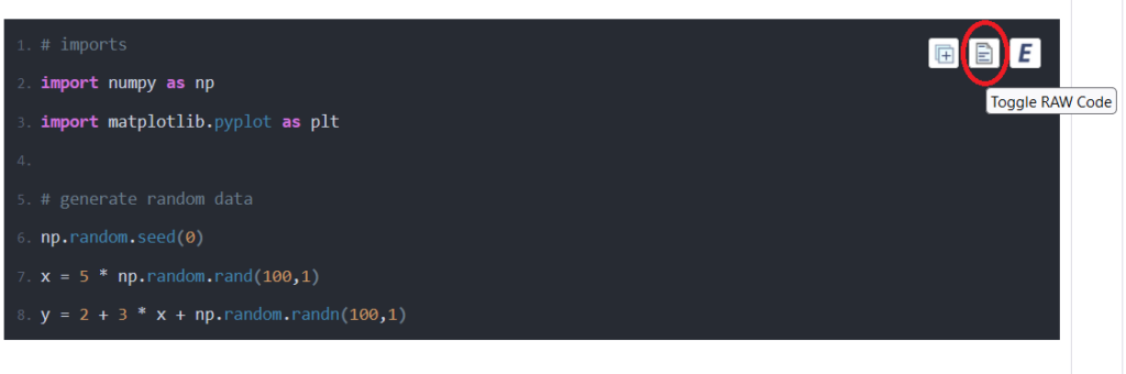
Copy and paste this code in your colab cell:

# imports
import numpy as np
import matplotlib.pyplot as plt

# generate random data
np.random.seed(0)
x = 5 * np.random.rand(100,1)
y = 2 + 3 * x + np.random.randn(100,1)

IMPORTANT!
You should pay attention to when you copy the code. You must click on the toggle button on the top right corner of the code as shown in the figure below to keep the correct indentation format. Otherwise, you must rearrange the format by yourself to have the correct indentation to avoid error in colab. Do the same to all the code you will copy.

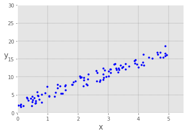
Here, we create a random dataset that spreads out along the line $y= 2+3x$ , where $\theta_0 = 2$ and $\theta_1 =3$ . This is a simple Linear regression problem with only one independent variable $\text{x}$ .

To be clear, we create our dataset randomly with the help of the line $y= 2+3x$ . Important to notice that here we pretend as if we didn’t know that our dataset was created from that line equation. So, our mission is to find the regression line based on the dataset that we have. You probably already know the answer. Yes, our regression line should be something close to line $y= 2+3x$ , where $\theta_0 \approx 2$ and $\theta_1 \approx 3$ .

Cool!

Ok, now you can print the shape of our data, and we have:

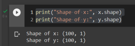
$\text{x}$ is a column vector of size $\text{100x1}$ and $\text{y}$ is also a column vector of size $\text{100x1}$ . This means that we have $100$ training examples $m$ .

We can be visualized our data using the following code, copy and paste it to your new colab cell and execute it.

plt.plot(x,y,'b.')
plt.xlabel("x", fontsize=15)
plt.ylabel("y", rotation=0, fontsize=15)
plt.grid(color = 'k', linestyle = '--', linewidth = 0.2)
_ =plt.axis([0,5.5,0,30])

That gives us this result:

Remember that a simple Linear regression model actually has two parameters, $\theta_0$ and $\theta_1$ . Therefore, we need to add a column of ones to the input $\text{x}$ dedicated to $x_0$ to deal with the intercept $\theta_0$ when we perform dot multiplication.

Simply copy and paste this code to your new colab cell to add a column of ones to the input $\text{x}$ .

#Add a column of ones
add_ones=np.ones((len(x), 1))
x_data=np.hstack((add_ones,x))
print("Shape of x_data:", x_data.shape)

After we add a column of ones to the $\text{x}$ , we can save it to another variable (x_data) to keep the original as it is. If you execute these lines, you have the output like this:

So now we have new data $\text{x_data}$ with dimensions of $\text{100x2}$ and $\text{y}$ with dimensions of $\text{100x1}$ .

GradientDescent function()

Nice! We already have our dataset and now we can write the Gradient descent function. To do so, we will implement Gradient descent (31) that we’ve just derived earlier.

Here is our GradientDescent() function. You can copy and paste it to a new cell:

def GradientDescent(X,y,theta,lr=0.01,n_iters=100):
    m = len(y)
    costs = [] 
    for _ in range(n_iters):
        y_hat = np.dot(X,theta)
        theta = theta -(1/m) * lr * (np.dot(X.T,(y_hat - y)))
        cost = (1/2*m) * np.sum(np.square(y_hat-y))
        costs.append(cost)
    return theta, costs

This function takes five input arguments as follows:
– x : input data,
– y : labels/actual values,
– theta : initial parameters $\bm{\theta}$ , initialized with random values,
– lr : learning rate ( $\alpha$ ), and
– n_iters : number of iterations.
and returns two variables, theta, and costs, where theta is the final updated parameters after reaching its maximum iteration and costs is the variable that keeps all the cost values during the iteration/learning process. Why do we need to keep the cost values? Well! we can plot them later on.

We’re going to break it down to better understanding of what we’re doing in the GradientDescent() function. As we know that Gradient descent algorithm calculates the gradient of the cost function and tweaks its parameters iteratively, so in line 4, we create a loop to update the parameters at every iteration step. We can specify the number of iterations n_iters for updating process.

    for _ in range(n_iters):

In line 5, we define the hypothesis (6), $h_{\bm{\theta}}(\text{x}) = \text{x}\bm{\theta}$ as y_hat:

        y_hat = np.dot(X,theta)

In line 6, we perform the update $\bm{\theta}$ as in (30), $\bm{\theta} & := \bm{\theta} - \frac{\alpha}{m} \left(\text{x}^T(\text{x}\bm{\theta}-\text{y})\right)$ :

        theta = theta -(1/m) * lr * (np.dot(X.T,(y_hat - y)))

Our cost function $J(\bm{\theta}) = \frac{1}{2m} \sum_{i=0}^m \Bigl( h_{\bm{\theta}}(\text{x}^{(i)})-\text{y}^{(i)} \Bigl)^2$ is written like this in the code (line 7):

        cost = (1/2*m) * np.sum(np.square(y_hat-y))

Ok, that’s it for the Gradient descent. And now we will be creating the LinearRegression() class.

Linear Regression Class

The following is the code for the LinearRegression() class. This class has three functions, __init__(), train(), and predict().

class LinearRegression:
    def __init__(self, lr=0.01, n_iters=1000):
        self.lr = lr
        self.n_iters = n_iters
        self.cost = np.zeros(self.n_iters)
        
    def train(self, x, y):
        self.theta =np.random.randn(x.shape[1],1)
        thetas,costs=GradientDescent(x,y,self.theta,self.lr,self.n_iters)
        self.theta=thetas
        self.cost=costs
        return self

    def predict(self, x):
        return np.dot(x, self.theta)

init() function

In the __init__() function, we set two input parameters, lr and n_iters. We also initialize a variable to store the history of the cost values, self.cost.

train() Function

In the train() function, we firstly initialize the self.theta with random values.

        self.theta =np.random.randn(x.shape[1],1)

Here, we define the self.theta with the shape of (x.shape[1],1). I hope you’re not get confused why we use the x.shape[1] instead of x_data.shape[1] here. x is actually an argument of train() function. When we call the train() function, we pass the argument x with x_data. So, the shape of x is actually the shape of x_data after we call the train() function. Since the shape of x_data is ( $100 x 2$ ). Then, the shape of self.theta will be ( $\text{2x1}$ ).

In line 9, we call the GradientDescent() function. .

        thetas,costs=GradientDescent(x,y,self.theta,self.lr,self.n_iters)

The GradientDescent() function returns the updated parameters (thetas) and the history of the cost (costs). We can the return all the values in line 12.

predict() function

In the predict() function, we simply calculate our hypothesis $h_{\bm{\theta}} (\text{x}) = \text{x}\bm{\theta}$ and return its value.

        return np.dot(x, self.theta)

Ok, that’s it for the LinearRegression() class! You see, it’s not too complicated, is it?

Now we have all the inggredients. so let’s finish it!.

Main Code

Ok, now we’re going to create our main code to solve our Linear regression problem.

Copy and paste this code to your new colab cell.

# Initialize the model
model = LinearRegression(lr=0.01, n_iters=1000)

# Train the data
model.train(x_data, y)

# printing thetas values
print('Thetas:' ,model.theta)

# Predict
y_predicted = model.predict(x_data)

# Plot original data points
plt.scatter(x, y, s=5,color='b')
plt.xlabel("x", fontsize=18)
plt.ylabel("y", rotation=0, fontsize=18)

# Draw predicted line
plt.plot(x, y_predicted, color='r')
_ =plt.axis([0,5.5,0,30])
plt.grid(color = 'k', linestyle = '--', linewidth = 0.2)
plt.show()

Line 2, we initialize the model by calling LinearRegression() class. Here, we can specify the learning rate lr and number of iteration n_iters as we need. You can experiment with that by trying different values and see what gives you.

model = LinearRegression(lr=0.01, n_iters=1000)

Line 5, we fit our training data to the model.

model.train(x_data, y)

Line 8, we print the paramaters theta. We should have two values for the theta, that are for $\theta_0$ and $\theta_1$ .

Line 11, we predict the data.

y_predicted = model.predict(x_data)

From lines 14 to 22, we plot the original data and the predicted line. That’s it for our main code.

Now we can execute this code and we got the result like this.

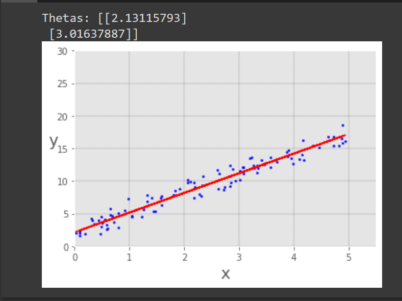
You see, here we have $\theta_0=2.13115793$ and $\theta_1=3.01637887$ . So our regression line is: $h_{\bm{\theta}}(\text{x})=2.13+3.02\text{x}$ , that’s pretty close to what we expected, $h_{\bm{\theta}}(\text{x})=2+3\text{x}$ .

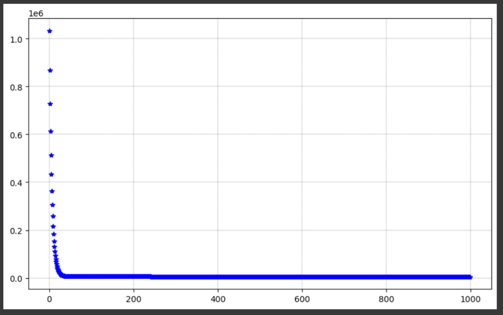
We can also plot the evolution of our cost like this:

cost=model.cost
# Plot cost 
plt.plot(range(len(cost)), cost, 'b*')
plt.grid(color = 'k', linestyle = '--', linewidth = 0.2)
plt.show()

And this is the plot of the evolution of the cost values.

Ok guys! This is the end of this tutorial. I hope you enjoy it.

Conclusion

You just learned about the Gradient descent and how to implement it in Python. You also learned about how to solve Linear regression problem using Gradient descent. I hope this tutorial is useful for developing your skills in Machine learning field. Don’t forget to share it and see you in the next tutorials.

I love sharing what I’ve learned to people. However, I cannot claim what I share is 100% accurate. If you know about something we missed or found something that is incorrect, please let me know by leaving your comments. That will improve my knowledge and help the community. Big thanks!.