Non-Maximum Suppression in PyTorch: How to Select the Correct Bounding Box

Posted by Rahmad Sadli on November 26, 2023 in Deep Learning, Machine Learning, Object Detection

Today, we will delve into the process of selecting the appropriate bounding box in object detection, focusing on the widely-used technique known as Non-Maximum Suppression (NMS). This tutorial will provide a comprehensive guide on implementing NMS in Python. By the end of this tutorial, you will not only understand the significance of choosing the right bounding box but also gain the practical know-how to seamlessly integrate Non-Maximum Suppression into your object detection pipeline 🚀👁️‍🗨️.

NMS Implementation Steps

Bounding boxes are essential elements in object detection used to localize objects within an image or video frame. The bounding box is typically defined by four elements that specify the position and size of the objects. It is commonly represented as ( $x, y, w, h$ ), where $x$ and $y$ denote the coordinates of the top-left corner, and $w$ and $h$ represent the width and height, respectively. Alternatively, it may be specified as ( $x_1, y_1, x_2, y_2$ ), where $x_1$ and $y_1$ indicate the coordinates of the top-left corner, and $x_2$ and $y_2$ denote the coordinates of the bottom-right corner.

In certain scenarios, object detection algorithms such as YOLO, Faster R-CNN, and SSD may generate redundant and overlapping bounding boxes. Therefore, to ensure accurate detection results and retain only the most confident ones, it is crucial to implement a mechanism capable of identifying and selecting the most appropriate bounding boxes while discarding the overlapping ones.

To achieve this objective, we can use a method called Non-Maximum Suppression (NMS), a post-processing technique commonly employed in object detection to suppress redundant or overlapping bounding boxes. When an object detection algorithm identifies multiple bounding boxes for the same object, NMS refines the results by retaining only the most accurate and relevant bounding box.

The implementation of NMS involves several steps, as follows:

Sort the bounding boxes based on their confidence scores in descending order.
Select the bounding box with the highest score as the proper bounding box.
Compare the selected bounding box with all the remaining boxes by calculating Intersection Over Union (IoU) scores. Set a predefined threshold for the IoU score. Bounding boxes with IoU scores above this threshold are considered overlapping.
Remove bounding boxes that significantly overlap with the selected bounding box (i.e., those with IoU scores above the threshold). This involves discarding lower-confidence boxes that contribute to the overlap. This method allows us to output only one proper bounding box for each detected object.
Save the selected bounding box to a selected bounding boxes list. This bounding box will be excluded from the next round.
Repeat the process from step 1 for the remaining bounding boxes list and always select the highest score as an appropriate bounding box. Continue until all bounding boxes are properly selected.

Alright! Now that we have the steps for processing NMS, we can proceed to the Python implementation. For this, we will use the bounding boxes produced by YOLOv3 prior to the NMS process.

Python Implementation

We will now explore an implementation example of using Non-Maximum Suppression in Python and PyTorch. For clarity, I have created two files: no_nms.py and with_nms.py. As the names suggest, no_nms.py aims to demonstrate the detection results produced by YOLOv3 prior to the NMS process, which may have overlapping bounding boxes for the same object. On the other hand, with_nms.py is the file where we apply NMS to eliminate the overlapping bounding boxes.

Great! Let’s now focus on the no_nms.py file first to gain insight into why we need the NMS process. In this example, we demonstrate the detection results without using the NMS technique.

#
# File name: no_nms.py
#

import matplotlib.pyplot as plt
import torch
from PIL import Image

# Define color list
colors_list = [
    (0.0, 0.0, 1.0),       # Blue
    (1.0, 0.0, 0.0),       # Red
    (0.0, 1.0, 0.0),       # Green 
    (1.0, 0.0, 1.0),       # Magenta
    (0.0, 1.0, 1.0),       # Cyan
    (1.0, 0.078, 0.576),   # Deep Pink    
    (0.502, 0.0, 0.0),     # Maroon
    (1.0, 1.0, 0.0),       # Yellow  
    (0.0, 0.502, 0.0),     # Green
    (1.0, 0.549, 0.412),   # Light Salmon
]

# Function for adding text to bounding boxes (to display conf score).        
def add_text(ax, text, position=(0, 0), box_color=(1, 1, 1, 0.7), text_color=(0, 0, 0), fontsize=12):
    ax.text(position[0], position[1], text,
            color=text_color, fontsize=fontsize,
            va='top', ha='left',
            bbox=dict(boxstyle="round,pad=0.1", linewidth=0, facecolor=box_color))


# Detection tensors obtained from YOLOv3 
detections = torch.tensor(
        [[ 1.7935e+02,  1.3099e+02,  2.5541e+02,  2.1599e+02,  9.9467e-01,  2.0000e+00],
        [ 1.8436e+02,  1.2741e+02,  2.6988e+02,  2.1938e+02,  5.3528e-01,  2.0000e+00],
        [ 1.0269e+02,  2.2538e+02,  2.1114e+02,  3.7338e+02,  9.9659e-01,  2.0000e+00],
        [ 9.8715e+01,  2.1940e+02,  2.1373e+02,  3.8053e+02,  9.9040e-01,  2.0000e+00],
        [ 1.0303e+02,  2.3210e+02,  2.1952e+02,  3.6961e+02,  9.5255e-01,  2.0000e+00],
        [ 1.0206e+02,  2.2447e+02,  2.2181e+02,  3.7882e+02,  9.3875e-01,  2.0000e+00],
        [ 4.3843e+02,  2.6350e+02,  5.6949e+02,  3.7186e+02,  6.9611e-01,  2.0000e+00],
        [ 4.4088e+02,  2.7646e+02,  5.7029e+02,  3.8060e+02,  9.9943e-01,  2.0000e+00],
        [ 4.4555e+02,  2.7596e+02,  5.8191e+02,  3.8002e+02,  9.7143e-01,  2.0000e+00],
        [ 1.1415e+02, -2.4183e-02,  1.7131e+02,  5.8423e+01,  9.1632e-01,  2.0000e+00],
        [ 1.2698e+02,  1.2038e-01,  1.7168e+02,  5.9562e+01,  8.9374e-01,  2.0000e+00],
        [ 1.2019e+02,  1.9048e-01,  1.7430e+02,  5.9384e+01,  9.9491e-01,  2.0000e+00],
        [ 4.0779e+01,  1.7749e+01,  7.9933e+01,  6.0788e+01,  9.4554e-01,  2.0000e+00],
        [ 3.8675e+01,  1.9767e+01,  8.1779e+01,  6.0434e+01,  9.9363e-01,  2.0000e+00],
        [ 1.1274e+02,  5.5822e-01,  1.7316e+02,  6.7431e+01,  7.5611e-01,  2.0000e+00],
        [ 1.2700e+02,  2.6155e+00,  1.7207e+02,  6.6231e+01,  7.3168e-01,  2.0000e+00],
        [ 1.2204e+02,  2.5143e+00,  1.7301e+02,  6.6141e+01,  9.8671e-01,  2.0000e+00],
        [ 1.1918e+02, -8.3912e-01,  1.7611e+02,  7.9783e+01,  5.5109e-01,  2.0000e+00],
        [ 1.3341e+02,  6.7477e+01,  1.8139e+02,  1.1677e+02,  8.7965e-01,  2.0000e+00],
        [ 1.3735e+02,  6.7784e+01,  1.8463e+02,  1.1717e+02,  5.8882e-01,  2.0000e+00],
        [ 1.3465e+02,  7.1647e+01,  1.8067e+02,  1.2851e+02,  9.6347e-01,  2.0000e+00],
        [ 1.3426e+02,  7.2629e+01,  1.8239e+02,  1.2802e+02,  9.9919e-01,  2.0000e+00],
        [ 1.3729e+02,  7.2342e+01,  1.8466e+02,  1.2793e+02,  5.0235e-01,  2.0000e+00],
        [ 1.3572e+02,  7.3281e+01,  1.8552e+02,  1.2820e+02,  9.8997e-01,  2.0000e+00],
        [ 4.3172e+01,  8.7346e+01,  1.0433e+02,  1.5540e+02,  9.5093e-01,  2.0000e+00],
        [ 4.5022e+01,  8.1346e+01,  1.0447e+02,  1.6264e+02,  9.9894e-01,  2.0000e+00],
        [ 4.8305e+01,  8.1125e+01,  1.1368e+02,  1.6075e+02,  6.4759e-01,  2.0000e+00],
        [ 1.8123e+02,  1.3002e+02,  2.5288e+02,  2.1806e+02,  9.9943e-01,  2.0000e+00],
        [ 1.8186e+02,  1.3412e+02,  2.5333e+02,  2.2153e+02,  9.9858e-01,  2.0000e+00],
        [ 4.1753e+01,  2.6930e+01,  7.9819e+01,  5.8917e+01,  9.2238e-01,  2.0000e+00]],
       device='cuda:0')


# Load image
image_path = "./image/test_image.jpg"
frame = Image.open(image_path)

# Input dimension YOLOv3 used to provide detections tensors for this example.
yolo_dim = (600, 600)


fig, ax = plt.subplots(figsize=(8, 6))
ax.imshow(frame)

for i, pred in enumerate(detections):
    boxes = pred[:4]
    scores = pred[4]    

    # Find the scale size between the output display and 
    # YOLOv3 input dimensions
    rw = frame.size[0] / yolo_dim[0]
    rh = frame.size[1] / yolo_dim[1]   

    x1y1 = (int(boxes[0] * rw), int(boxes[1] * rh))
    x2y2 = (int(boxes[2] * rw), int(boxes[3] * rh))
    
    rect = plt.Rectangle(x1y1, x2y2[0] - x1y1[0], x2y2[1] - x1y1[1], linewidth=2,
                         edgecolor=colors_list[i%10], facecolor='none')
    ax.add_patch(rect)

    txt = f"Score: {round(float(scores), 2)}"
    add_text(ax, txt, position=x1y1, box_color=(colors_list[i%10], 0.4), text_color=(1, 1, 1), fontsize=12)

plt.show()

In this code, we use a tensor of detections generated by YOLOv3, as presented below:

detections = torch.tensor(
        [[ 1.7935e+02,  1.3099e+02,  2.5541e+02,  2.1599e+02,  9.9467e-01,  2.0000e+00],
        [ 1.8436e+02,  1.2741e+02,  2.6988e+02,  2.1938e+02,  5.3528e-01,  2.0000e+00],
        [ 1.0269e+02,  2.2538e+02,  2.1114e+02,  3.7338e+02,  9.9659e-01,  2.0000e+00],
        [ 9.8715e+01,  2.1940e+02,  2.1373e+02,  3.8053e+02,  9.9040e-01,  2.0000e+00],
        [ 1.0303e+02,  2.3210e+02,  2.1952e+02,  3.6961e+02,  9.5255e-01,  2.0000e+00],
        [ 1.0206e+02,  2.2447e+02,  2.2181e+02,  3.7882e+02,  9.3875e-01,  2.0000e+00],
        [ 4.3843e+02,  2.6350e+02,  5.6949e+02,  3.7186e+02,  6.9611e-01,  2.0000e+00],
        [ 4.4088e+02,  2.7646e+02,  5.7029e+02,  3.8060e+02,  9.9943e-01,  2.0000e+00],
        [ 4.4555e+02,  2.7596e+02,  5.8191e+02,  3.8002e+02,  9.7143e-01,  2.0000e+00],
        [ 1.1415e+02, -2.4183e-02,  1.7131e+02,  5.8423e+01,  9.1632e-01,  2.0000e+00],
        [ 1.2698e+02,  1.2038e-01,  1.7168e+02,  5.9562e+01,  8.9374e-01,  2.0000e+00],
        [ 1.2019e+02,  1.9048e-01,  1.7430e+02,  5.9384e+01,  9.9491e-01,  2.0000e+00],
        [ 4.0779e+01,  1.7749e+01,  7.9933e+01,  6.0788e+01,  9.4554e-01,  2.0000e+00],
        [ 3.8675e+01,  1.9767e+01,  8.1779e+01,  6.0434e+01,  9.9363e-01,  2.0000e+00],
        [ 1.1274e+02,  5.5822e-01,  1.7316e+02,  6.7431e+01,  7.5611e-01,  2.0000e+00],
        [ 1.2700e+02,  2.6155e+00,  1.7207e+02,  6.6231e+01,  7.3168e-01,  2.0000e+00],
        [ 1.2204e+02,  2.5143e+00,  1.7301e+02,  6.6141e+01,  9.8671e-01,  2.0000e+00],
        [ 1.1918e+02, -8.3912e-01,  1.7611e+02,  7.9783e+01,  5.5109e-01,  2.0000e+00],
        [ 1.3341e+02,  6.7477e+01,  1.8139e+02,  1.1677e+02,  8.7965e-01,  2.0000e+00],
        [ 1.3735e+02,  6.7784e+01,  1.8463e+02,  1.1717e+02,  5.8882e-01,  2.0000e+00],
        [ 1.3465e+02,  7.1647e+01,  1.8067e+02,  1.2851e+02,  9.6347e-01,  2.0000e+00],
        [ 1.3426e+02,  7.2629e+01,  1.8239e+02,  1.2802e+02,  9.9919e-01,  2.0000e+00],
        [ 1.3729e+02,  7.2342e+01,  1.8466e+02,  1.2793e+02,  5.0235e-01,  2.0000e+00],
        [ 1.3572e+02,  7.3281e+01,  1.8552e+02,  1.2820e+02,  9.8997e-01,  2.0000e+00],
        [ 4.3172e+01,  8.7346e+01,  1.0433e+02,  1.5540e+02,  9.5093e-01,  2.0000e+00],
        [ 4.5022e+01,  8.1346e+01,  1.0447e+02,  1.6264e+02,  9.9894e-01,  2.0000e+00],
        [ 4.8305e+01,  8.1125e+01,  1.1368e+02,  1.6075e+02,  6.4759e-01,  2.0000e+00],
        [ 1.8123e+02,  1.3002e+02,  2.5288e+02,  2.1806e+02,  9.9943e-01,  2.0000e+00],
        [ 1.8186e+02,  1.3412e+02,  2.5333e+02,  2.2153e+02,  9.9858e-01,  2.0000e+00],
        [ 4.1753e+01,  2.6930e+01,  7.9819e+01,  5.8917e+01,  9.2238e-01,  2.0000e+00]],
       device='cuda:0')

Here, each column of the detections tensor corresponds to the following information:

| $x_1$ | $y_1$ | $x_2$ | $y_2$ | conf_score | class_id |

These detections were extracted from the output of YOLOv3 before the NMS process. As you’ll observe shortly, even though these detections have been filtered with a confidence threshold value of 0.5, each detected object is still associated with more than one bounding box. Hence, we need to eliminate these unnecessary bounding boxes to ensure that each object is assigned only the most appropriate bounding box.

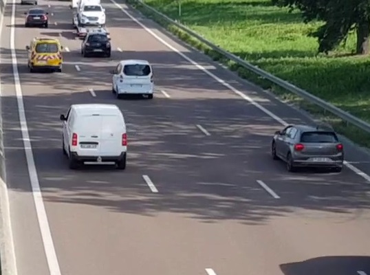
You can simply right-click and save the following image to your image folder to test the code. Don’t forget to change the image path to where you save this image in this line:

image_path = "./image/test_image.jpg"

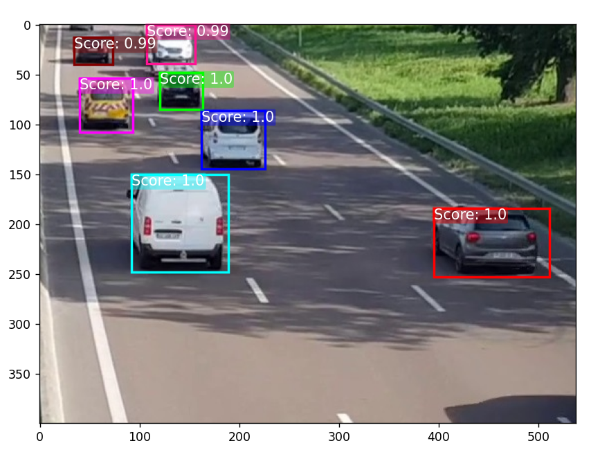
Here is the output of the code.

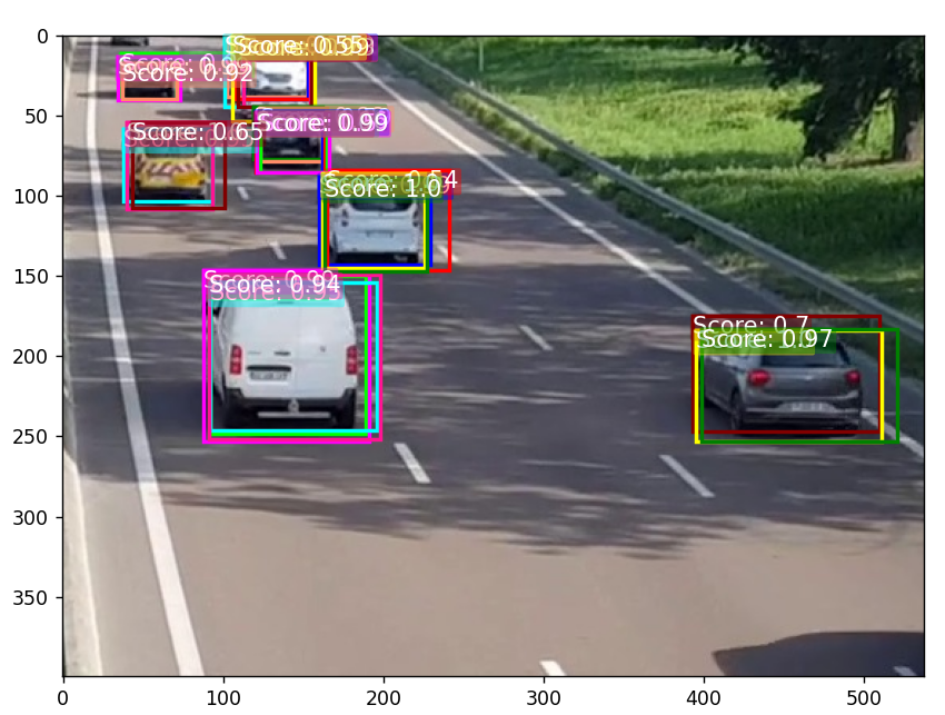
As you can see, each detected object has multiple bounding boxes. To address this, we need to apply the Non-Maximum Suppression process to select the most appropriate bounding box for each object.

Copy and paste the following code into your code editor.

"""
with_nms.py
"""

import matplotlib.pyplot as plt
import torch
from PIL import Image

# Define color list
colors_list = [
    (0.0, 0.0, 1.0),       # Blue
    (1.0, 0.0, 0.0),       # Red
    (0.0, 1.0, 0.0),       # Green 
    (1.0, 0.0, 1.0),       # Magenta
    (0.0, 1.0, 1.0),       # Cyan
    (1.0, 0.078, 0.576),   # Deep Pink    
    (0.502, 0.0, 0.0),     # Maroon
    (1.0, 1.0, 0.0),       # Yellow  
    (0.0, 0.502, 0.0),     # Green
    (1.0, 0.549, 0.412),   # Light Salmon
]

# Function for adding text to bounding boxes (to display conf score).    
def add_text(ax, text, position=(0, 0), box_color=(1, 1, 1, 0.7), text_color=(0, 0, 0), fontsize=12):
    ax.text(position[0], position[1], text,
            color=text_color, fontsize=fontsize,
            va='top', ha='left',
            bbox=dict(boxstyle="round,pad=0.1", linewidth=0, facecolor=box_color))

# Detection tensors obtained from YOLOv3    
detections = torch.tensor(
        [[ 1.7935e+02,  1.3099e+02,  2.5541e+02,  2.1599e+02,  9.9467e-01,  2.0000e+00],
        [ 1.8436e+02,  1.2741e+02,  2.6988e+02,  2.1938e+02,  5.3528e-01,  2.0000e+00],
        [ 1.0269e+02,  2.2538e+02,  2.1114e+02,  3.7338e+02,  9.9659e-01,  2.0000e+00],
        [ 9.8715e+01,  2.1940e+02,  2.1373e+02,  3.8053e+02,  9.9040e-01,  2.0000e+00],
        [ 1.0303e+02,  2.3210e+02,  2.1952e+02,  3.6961e+02,  9.5255e-01,  2.0000e+00],
        [ 1.0206e+02,  2.2447e+02,  2.2181e+02,  3.7882e+02,  9.3875e-01,  2.0000e+00],
        [ 4.3843e+02,  2.6350e+02,  5.6949e+02,  3.7186e+02,  6.9611e-01,  2.0000e+00],
        [ 4.4088e+02,  2.7646e+02,  5.7029e+02,  3.8060e+02,  9.9943e-01,  2.0000e+00],
        [ 4.4555e+02,  2.7596e+02,  5.8191e+02,  3.8002e+02,  9.7143e-01,  2.0000e+00],
        [ 1.1415e+02, -2.4183e-02,  1.7131e+02,  5.8423e+01,  9.1632e-01,  2.0000e+00],
        [ 1.2698e+02,  1.2038e-01,  1.7168e+02,  5.9562e+01,  8.9374e-01,  2.0000e+00],
        [ 1.2019e+02,  1.9048e-01,  1.7430e+02,  5.9384e+01,  9.9491e-01,  2.0000e+00],
        [ 4.0779e+01,  1.7749e+01,  7.9933e+01,  6.0788e+01,  9.4554e-01,  2.0000e+00],
        [ 3.8675e+01,  1.9767e+01,  8.1779e+01,  6.0434e+01,  9.9363e-01,  2.0000e+00],
        [ 1.1274e+02,  5.5822e-01,  1.7316e+02,  6.7431e+01,  7.5611e-01,  2.0000e+00],
        [ 1.2700e+02,  2.6155e+00,  1.7207e+02,  6.6231e+01,  7.3168e-01,  2.0000e+00],
        [ 1.2204e+02,  2.5143e+00,  1.7301e+02,  6.6141e+01,  9.8671e-01,  2.0000e+00],
        [ 1.1918e+02, -8.3912e-01,  1.7611e+02,  7.9783e+01,  5.5109e-01,  2.0000e+00],
        [ 1.3341e+02,  6.7477e+01,  1.8139e+02,  1.1677e+02,  8.7965e-01,  2.0000e+00],
        [ 1.3735e+02,  6.7784e+01,  1.8463e+02,  1.1717e+02,  5.8882e-01,  2.0000e+00],
        [ 1.3465e+02,  7.1647e+01,  1.8067e+02,  1.2851e+02,  9.6347e-01,  2.0000e+00],
        [ 1.3426e+02,  7.2629e+01,  1.8239e+02,  1.2802e+02,  9.9919e-01,  2.0000e+00],
        [ 1.3729e+02,  7.2342e+01,  1.8466e+02,  1.2793e+02,  5.0235e-01,  2.0000e+00],
        [ 1.3572e+02,  7.3281e+01,  1.8552e+02,  1.2820e+02,  9.8997e-01,  2.0000e+00],
        [ 4.3172e+01,  8.7346e+01,  1.0433e+02,  1.5540e+02,  9.5093e-01,  2.0000e+00],
        [ 4.5022e+01,  8.1346e+01,  1.0447e+02,  1.6264e+02,  9.9894e-01,  2.0000e+00],
        [ 4.8305e+01,  8.1125e+01,  1.1368e+02,  1.6075e+02,  6.4759e-01,  2.0000e+00],
        [ 1.8123e+02,  1.3002e+02,  2.5288e+02,  2.1806e+02,  9.9943e-01,  2.0000e+00],
        [ 1.8186e+02,  1.3412e+02,  2.5333e+02,  2.2153e+02,  9.9858e-01,  2.0000e+00],
        [ 4.1753e+01,  2.6930e+01,  7.9819e+01,  5.8917e+01,  9.2238e-01,  2.0000e+00]],
       device='cuda:0')


# IoU calculation function
def bbox_ious(box1, box2):
    x1 = torch.max(box1[:, 0], box2[:, 0])
    y1 = torch.max(box1[:, 1], box2[:, 1])
    x2 = torch.min(box1[:, 2], box2[:, 2])
    y2 = torch.min(box1[:, 3], box2[:, 3])

    inter_area = torch.clamp(x2 - x1, min=0) * torch.clamp(y2 - y1, min=0)

    area_box1 = (box1[:, 2] - box1[:, 0]) * (box1[:, 3] - box1[:, 1])
    area_box2 = (box2[:, 2] - box2[:, 0]) * (box2[:, 3] - box2[:, 1])

    iou = inter_area / (area_box1 + area_box2 - inter_area)

    return iou

# non-maximum suppression function
def non_max_suppresion(prediction, iou_threshold):
    boxes = prediction[:, :4]
    scores = prediction[:, 4]        

    sorted_indices = torch.argsort(scores, descending=True)

    boxes = boxes[sorted_indices]
    scores = scores[sorted_indices]

    selected_indices = []
    
    while(boxes.size(0)>0):        
        
        selected_box = boxes[0]        
        selected_indices.append(sorted_indices[0])            

        ious = bbox_ious(selected_box.unsqueeze(0), boxes[1:])
        mask = ious < iou_threshold 

        boxes = boxes[1:][mask]
        scores = scores[1:][mask]
        sorted_indices = sorted_indices[1:][mask]   
                
        
    selected_indices = torch.tensor(selected_indices, dtype=torch.long)

    nms_pred = prediction[selected_indices]        
    return nms_pred


# Load image
image_path = "./image/test_image.jpg"
frame = Image.open(image_path)

# The input dimension of YOLOv3 that was used to generate the detection tensors in this example.
yolo_dim = (600, 600)

# call the non_max_suppression function with IoU threshold= 0.5
detections = non_max_suppresion(detections, 0.5)

# Plot the result
fig, ax = plt.subplots(figsize=(8, 8))
ax.imshow(frame)

for i, pred in enumerate(detections):
    boxes = pred[:4]  
    scores = pred[4]    

    # Find the scale size between the output display and 
    # YOLOv3 input dimensions
    rw = frame.size[0] / yolo_dim[0]
    rh = frame.size[1] / yolo_dim[1]   

    x1y1 = (int(boxes[0] * rw), int(boxes[1] * rh))
    x2y2 = (int(boxes[2] * rw), int(boxes[3] * rh))
    
    rect = plt.Rectangle(x1y1, x2y2[0] - x1y1[0], x2y2[1] - x1y1[1], linewidth=2,
                         edgecolor=colors_list[i%10], facecolor='none')
    ax.add_patch(rect)

    txt = f"Score: {round(float(scores), 2)}"
    add_text(ax, txt, position=x1y1, box_color=(colors_list[i%10], 0.4), text_color=(1, 1, 1), fontsize=12)

plt.show()

Great! Before we execute this program, let’s take a closer look at the non_max_suppression() function as follows::

Lines 83-84: Extract bounding boxes and scores from the prediction tensor. The first four columns are the coordinates ( $x_1, y_1, x_2, y_2$ ) of the bounding boxes, and the fifth column represents the confidence scores of the bounding boxes.

    boxes = prediction[:, :4]
    scores = prediction[:, 4]

Line 86: Sort the elements of the scores tensor in descending order and save the resulting indices in the variable sorted_indices.

    sorted_indices = torch.argsort(scores, descending=True)

Line 88-89: Reorder the boxes and scores tensors based on the sorted indices. Now, both the boxes and scores are aligned in descending order of the confidence scores.

    boxes = boxes[sorted_indices]
    scores = scores[sorted_indices]

Line 91: Initialize an empty list to store selected indices

Line 93: Loop over the bounding boxes:

Line 95: Select the bounding box with the highest score. Since we already aligned the boxes tensor in decending order of confidence scores, the bounding box which corresponds to the highest confidence score it boxes[0].

        selected_box = boxes[0]

Line 96: Append the index that corresponds to the highest confidence score (sorted_indices[0]) to the selected_indices list.

        selected_indices.append(sorted_indices[0])

Line 98 - 99: Calculate the IoU between the selected bounding box and the remaining bounding boxes. Then, filter out bounding boxes with an IoU greater than the specified threshold (iou_threshold) using a boolean mask (mask). The mask is set to True for bounding boxes where the IoU is less than the specified threshold.

        ious = bbox_ious(selected_box.unsqueeze(0), boxes[1:])
        mask = ious < iou_threshold

Lines 101 - 103: Update boxes, scores, and sorted_indices based on the provided boolean mask. The updated values exclude the first index, which corresponds to the bounding box that has just been selected.

        boxes = boxes[1:][mask]
        scores = scores[1:][mask]
        sorted_indices = sorted_indices[1:][mask]

Line 106: Convert the list of selected indices to a tensor.

    selected_indices = torch.tensor(selected_indices, dtype=torch.long)

Line 108: Select the boxes with the selected indices from the original prediction tensor to get the final NMS result.

    nms_pred = prediction[selected_indices]

Line 109: Return the final NMS result.

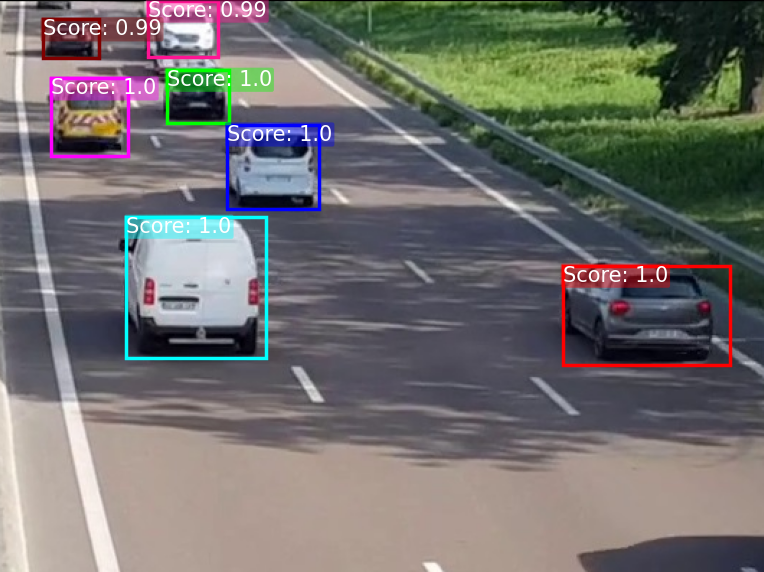
Fantastic! Now you can execute the code. The result, as shown in the figure below, demonstrates that the redundant bounding boxes have been completely removed. NMS has already selected the best bounding box, which has the highest confidence score for each object.

Conclusion

You have just completed the tutorial on Non-Maximum Suppression. By reaching this point, I hope you now have a clear understanding of how NMS works and are capable of implementing it in your own object detection pipeline. Best of luck to you, and don’t forget to check out my other tutorials.

Non-Maximum Suppression in PyTorch: How to Select the Correct Bounding Box

NMS Implementation Steps

Python Implementation

Conclusion

Recently Posted Tutorials

Populer Tutorials

Leave a Reply Cancel reply