Introduction to Multi-Object Tracking (MOT)

Posted by Rahmad Sadli on December 18, 2023 in Multi-Object Tracking, Object Tracking

Previously, we learned how to implement the 2-D Kalman filter to track a single moving object, effectively estimating its positions in 2-D space. Today, we’ll explore a special topic in object tracking—Multi-Object Tracking (MOT).

Without further ado, let’s begin this discussion.

Introduction

Multi-Object Tracking (MOT) is an essential task in computer vision that involves tracking multiple objects in both recorded videos and real-time live-streaming scenarios. As a longstanding goal in computer vision and machine learning, MOT is becoming increasingly important and widely applied in various fields, including autonomous driving, traffic monitoring and flow counting, and many more.

MOT plays a crucial role in autonomous driving. Its primary function involves tracking the trajectories of other vehicles, vulnerable road users such as cyclists and pedestrians, as well as other objects on the road. This information is then utilized by autonomous vehicles to execute secure and efficient driving maneuvers.

For instance, when an autonomous car detects pedestrians crossing the road, the MOT system tracks their positions and velocities to predict their future movements. This information guides the car’s planning and control algorithms in adjusting the vehicle’s speed and trajectory to avoid potential collisions.

Similarly, when the autonomous car detects another vehicle in its vicinity, the tracking system provides information about the position, speed, and heading of that vehicle. This data is then used by the autonomous car’s planning and control algorithms to adjust its own speed and heading, ensuring a safe distance is maintained and potential collisions can be avoided.

In traffic monitoring and flow counting, MOT can offer valuable insights into traffic patterns, congestion, and accidents. It plays a crucial role in flow counting by enhancing vehicle counting through the tracking of vehicle trajectories near the counting line. By monitoring the trajectories of various objects, including vehicles and pedestrians, MOT captures detailed information about traffic patterns, congestion dynamics, and accident occurrences. This invaluable data not only deepens our understanding of road usage but also empowers urban planners and traffic management authorities to formulate more efficient and safer transportation strategies.

Challenges in Multi-Object Tracking

In recent years, MOT has drawn growing interest due to its potential in both academic research and commercial applications within the field of computer vision. However, the task of MOT remains challenging due to various factors. MOT involves simultaneously handling multiple objects, tracking their positions, and monitoring their interactions. The system must also maintain a consistent track identity for the same object from its initial detection, deal with abrupt appearance changes and severe object occlusions. Moreover, it needs to address other complex scenarios, such as objects entering and exiting the scene.

To address these challenges and enhance the accuracy and robustness of MOT systems, researchers have developed various algorithms and techniques, including filter-based, graph-based, and deep learning-based methods, each with its own set of advantages and limitations.

Why is Multi-Object Tracking necessary?

As computer vision and machine learning continue to advance, MOT has become an increasingly powerful tool for analyzing and understanding complex visual data. However, some may question why MOT is necessary for tracking objects when the object detection algorithm seems sufficient.

It is important to understand that object detection and MOT serve different purposes in computer vision. Object detection aims to detect the presence and location of objects in images or videos. Even though this is a crucial component of many computer vision applications, object detection alone cannot provide a complete understanding of an object’s behavior or motion. For instance, in a traffic monitoring system, object detection can detect the presence of a vehicle, but it cannot provide information about the vehicle’s trajectory and speed. To obtain this information, MOT is necessary.

The goal of MOT is to track objects over time as they move through a scene, identify and distinguish them from other objects in the same frame. MOT allows us to track the movements and trajectories of multiple objects over time and associate them with their respective identities. This information can be analyzed to gain insights into their behaviors, predict their future movements, and identify patterns in their motions.

Integrating MOT with object detection can provide more accurate and reliable results compared to object detection alone, especially in crowded and complex scenarios where objects may occlude each other, move in and out of the frame, or change appearance. By integrating MOT with object detection, we can obtain a more comprehensive understanding of the scene and improve the performance of various computer vision tasks.

Great! Let’s now discuss one of the challenging tasks in MOT, Track association.

Track Association

The components involved in Multi-Object Tracking (MOT) are similar to those in single-object tracking, including observation, prediction, and estimation. However, MOT presents a more complex problem as it involves simultaneously tracking multiple objects. It requires correctly associating existing tracks with their corresponding new detections.

The process of associating existing tracks with new detections is called track association. It involves assigning the existing tracks estimated at time 𝑡 − 1 to the current detections at time 𝑡.

Track association is one of the most significant challenges in MOT because it involves tracking targets moving in random directions with varying velocities. Furthermore, the number of new observations can vary compared to existing tracks due to objects entering and exiting the scene or possibly being occluded or overlap with each other. These factors add complexity to the task of track association. It’s important to note that this association must adhere to the constraint that each track can only be assigned to one detection and vice versa.

Having a reliable and efficient track association algorithm is essential to ensure the optimal performance of an MOT system because inaccurate track association can lead to lost tracks or even the creation of new tracks for the same objects that were being tracked in the previous frames.

Alright! Now, let’s continue to understand how track association can be formulated.

Problem Formulation

For a better understanding of the track association problem in Multi-Object Tracking, let’s focus on the following simplified cases in MOT. For simplicity, we assume perfect detector performance with no false negatives or false positives.

Suppose that at time 𝑡 − 1, we have three existing tracks labeled as 𝑇1, 𝑇2, and 𝑇3. Then, at time 𝑡, various detection combinations can arise, as illustrated by these potential examples:

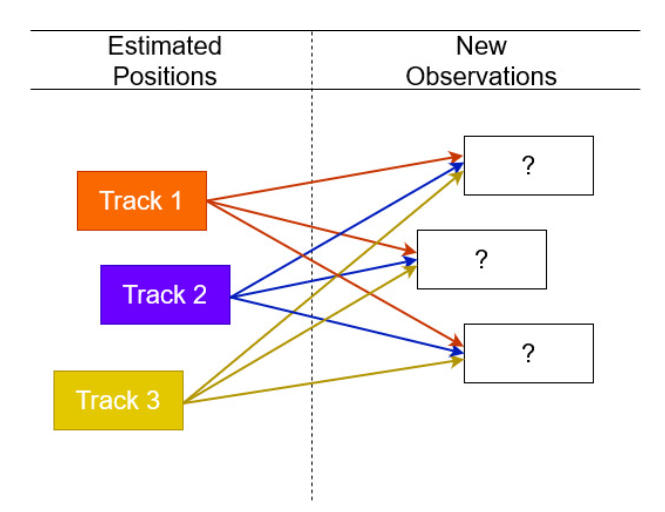
Case 1: The detector detects three targets at the current time 𝑡, which is the same as the number of existing tracks at the previous time 𝑡 − 1, as illustrated in the figure below.

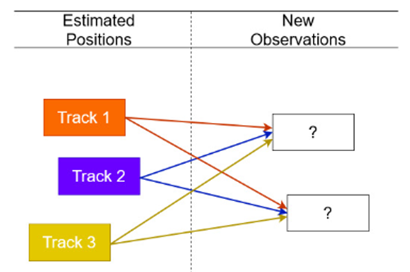
Case 2: One of the targets has vanished from the scene, and the detector accurately identifies that there are two targets at the current time 𝑡, as shown in the figure below.

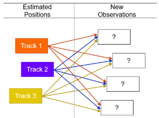
Case 3: A new target appears in the scene, and the detector correctly detects that there are four targets at the current time 𝑡, as depicted in the figure below.

The examples presented above show the significant challenge of associating the existing tracks with their corresponding detections in Multi-Object Tracking. As demonstrated in these examples, it is highly challenging to accurately determine which track corresponds to the correct detection. Therefore, an effective optimization method is necessary. To find the optimal solution for the track association problem, we can formulate the problem as follows:

Given the cost matrix C = [𝑐_𝑖𝑗], where 𝑐_𝑖𝑗 represents the cost of assigning track 𝑖 to detection 𝑗, find the matrix 𝑋 = [𝑥_𝑖𝑗] such that:

(1) $\begin{equation*}\boxed{ \textcolor{black} {\sum^n_{i=1} \sum^m_{j=1} c_{ij} x_{ij}}}\end{equation*}$

is minimized, subject to:

(2) $\begin{equation*}\begin{split}\sum_i x_{ij} &= 1, \quad \forall j \\\sum_j x_{ij} &= 1, \quad \forall i\end{split}\end{equation*}$

The variable 𝑥_𝑖𝑗 is binary, which ensures each detection is associated with one and only one track and each track is associated with one and only one detection. Therefore, 𝑥_𝑖𝑗 must be either 0 or 1, i.e., 𝑥_𝑖𝑗 ∈ 0, 1.

Now that we have formulated the problem of obtaining the optimal solution for track association, an essential element emerges—the cost matrix. What role does the cost matrix play in track association? Let’s continue this discussion to understand its significance and learn how to construct it, as it plays a crucial part in this process.

Cost Matrix

The cost matrix is a vital component in optimizing the track association problem in Multi-Object Tracking. It is a two-dimensional matrix where each element represents the cost of assigning a track to a new detection. In other words, each row of the cost matrix represents a track, while each column represents a new detection.

The cost of assigning existing tracks to new detections in Multi-Object Tracking can be calculated using various metrics, such as distance, Intersection over Union (IoU), and appearance similarity. Selecting the appropriate metric for generating a cost matrix is crucial for achieving optimal tracking performance. The choice of metric depends on the characteristics of the objects that will be tracked and the specific requirements of a tracking system.

In this post, we will use a simple yet popular metric—Euclidean distance to create a cost matrix. The Euclidean distance can be calculated directly between two points or, in the tracking paradigm, between the center of the actual object position and the center of its next predicted position.

The Euclidean distance 𝐸_{𝑑𝑖𝑠𝑡} between two points (𝑥_𝑎, 𝑦_𝑎) and 𝐵(𝑥_𝑏, 𝑦_𝑏) is calculated as follows:

(3) $\begin{equation*}\boxed{ \textcolor{black} {E_{dist} = \sqrt{(x_b - x_a)^2 + (y_b - y_a)^2}}}\end{equation*}$

Example 1.

For a better understanding of how to construct the cost matrix, let’s look at the following example of a track association problem presented in the figure below.

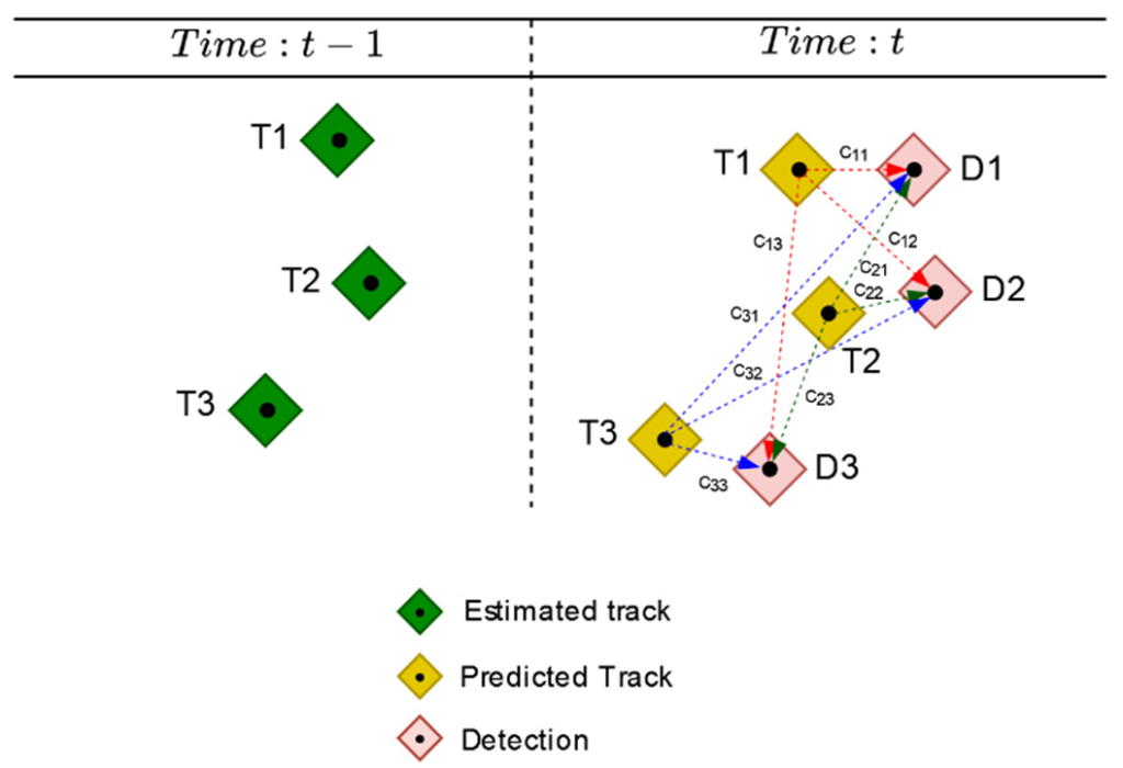
Tracking Muti-Object: Track Association problem

In this illustration, there are three estimated tracks at time 𝑡 − 1, as well as three new detections and three predicted tracks at time 𝑡.

For this association case, we create a 3 × 3 cost matrix denoted as C, which represents the costs of each potential association. Each element 𝑐_𝑖𝑗 in the matrix corresponds to the cost of assigning a track to a new detection. Specifically, 𝑐_𝑖𝑗 represents the cost of assigning the 𝑖-th track to the 𝑗-th detection. For instance, 𝑐₁₂ signifies the cost of assigning the first track to the second detection, and 𝑐₃₃ represents the cost of assigning the third track to the third detection.

It’s important to note that the cost matrix is calculated based on the positions of predicted tracks and new detections.

You can find the following pseudocode for creating a matrix using the Euclidean distance.

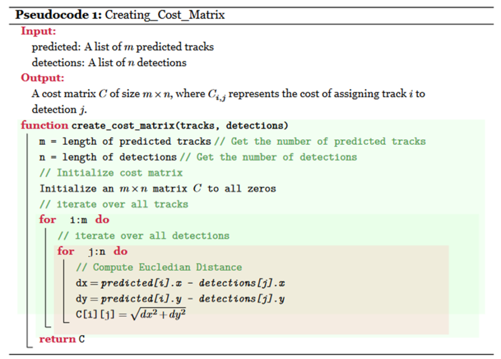
Mutli-Object Tracking: Cost Matrix Pseudo Code

This pseudocode defines a function that takes two inputs: a list of predicted tracks and a list of detections. It then outputs a cost matrix, where each element represents the cost of assigning a predicted track to a detection. The algorithm initializes a matrix of zeros with the same size as the output cost matrix. It then iterates over all possible pairs and computes the Euclidean distance between each predicted track and each detection in the pair. The distance is assigned to the corresponding element of the cost matrix, denoted as C_𝑖𝑗. Finally, the function returns the cost matrix C as its output.

Example 2.

This example provides a more practical approach because we will generate a cost matrix using the pseudo-code above.

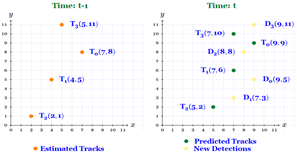
Multi-Object Tracking: Example Track Association

Look at the scenario illustrated in the figure above. At time 𝑡 − 1, there are four estimated tracks represented by orange circles. At time 𝑡, we have four predicted tracks represented by green circles and four new detections represented by yellow circles.

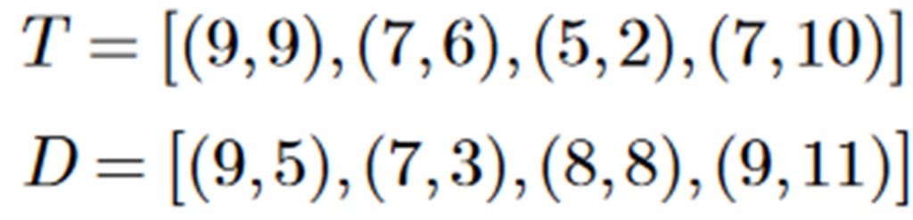
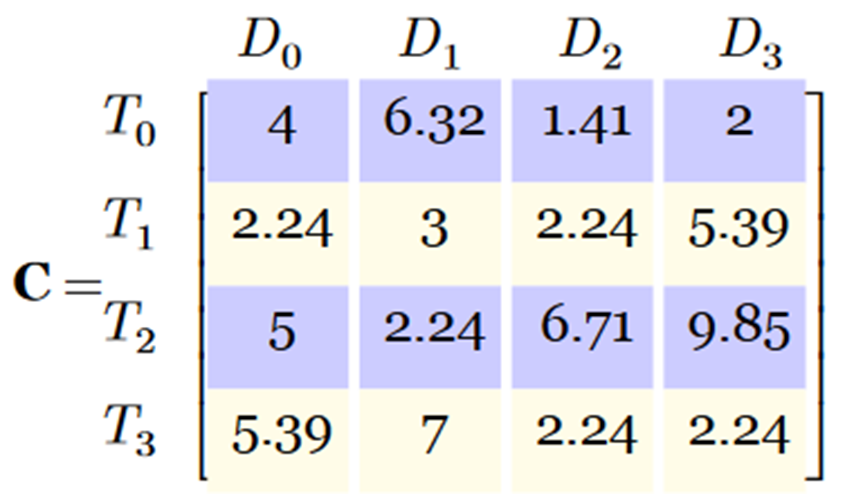
Let’s generate the cost matrix for this scenario. As shown in the figure above, at time 𝑡, there are four predicted tracks 𝑇0, 𝑇1, 𝑇2, 𝑇3, and four detections 𝐷0, 𝐷1, 𝐷2, 𝐷3. The list of coordinates for both predicted tracks (𝑇) and detections (𝐷) is as follows:

Then, we implement the pseudo-code 1 into Python code as follows:

import numpy as np

def generate_cost_matrix(pred_tracks, detections):
    """
    Input: -pred_tracks: list of the predicted_tracks, 
           -detections: list of detections
    Output: cost_matrix
    """
    n = len(pred_tracks)
    m = len(detections)
    
    #initialize cost_matrix to zeros
    cost_matrix = np.zeros((m, n))    
    for i in range(n):        
        for j in range(m):
            dx = pred_tracks[i][0] - detections[j][0]
            dy = pred_tracks[i][1] - detections[j][1]
            distance = np.sqrt(dx**2 + dy**2)
            cost_matrix[i][j]=round(distance, 2)            
    return cost_matrix

#Define list of predicted tracks (PT) and detections (D)
T = [(9, 9), (7, 6), (5, 2), (7,10)]
D = [(9, 5), (7,3), (8,8),(9,11)]
# Execute generate_cost_matrix() function
cost_matrix =generate_cost_matrix(T,D)
print(cost_matrix)

This code produces the following result:

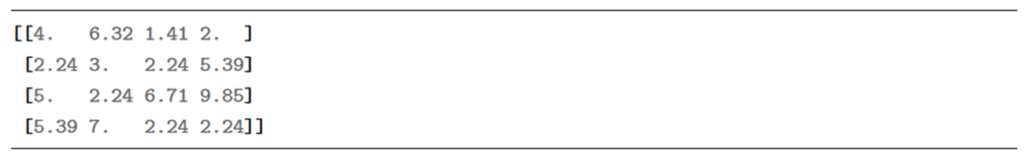
This means that, we have a 4 × 4 cost matrix C as follows:

Great! By now, you should have a solid understanding of the track association problem and the process of creating a cost matrix using Euclidean distance. The next step is to explore the algorithms available to solve the track assignment problem by minimizing the cost matrix.

For a smaller cost matrix, the Brute-force method offers a straightforward approach to explore all potential solutions and identify the optimal one. In general, an 𝑛 × 𝑛 cost matrix has 𝑛! possible solutions. For example, a 3×3 cost matrix has 6 potential solutions, a 4×4 cost matrix has 24, and so on. However, as the cost matrix grows, and the solution space increases factorially, the Brute-force method quickly becomes computationally expensive and is definitely unsuitable for real-time applications.

Therefore, it’s essential to find a more efficient algorithm for solving the track association problem. One of the widely used algorithms for this purpose is the Hungarian algorithm. This algorithm is based on the principle of iterative improvement and can solve the problem in 𝑂(𝑛 $^3$ ) time. This makes it much faster than the Brute-force method for larger values of 𝑛.

You can learn more about Track Association with the Hungarian algorithm by simply grabbing my eBook, ‘Beginner’s Guide to Multi-Object Tracking with Kalman Filter.’ This book will guide you through a deeper understanding of the Hungarian algorithm and demonstrate how to use it to optimize the track association problem with examples.

You can grab it for only $10, and it covers everything you need to know to implement a Multi-Object Tracking system in Python.

What do you get after purchasing this eBook?

A copy of the eBook in PDF format
The complete implementation code in a ZIP file with testing videos.

Grab it now with 25% OFF with coupon code: MIJY159IMW

Free preview: