Introduction to Artiﬁcial Neural Networks (ANNs)

Posted by Rahmad Sadli on February 7, 2020 in Deep Learning, Machine Learning

Artiﬁcial Neural Networks (ANNs), inspired by the human brain system, are based on a collection of units of neurons that are connected one to another to process and send information.

A very basic or a simplest neural network composes of only a single neuron, some inputs $\textbf{x} = (x_1, x_2,..,x_n)$ and a bias b as illustrated in the following ﬁgure.

Neural Networks: a simplest neural network

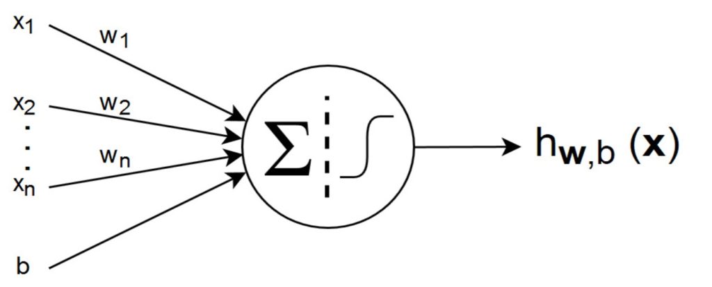
All the inputs and the bias are connected to this neuron. These connections are called the synapses where every synapse has the weight W.

The hypothesis output of this simplest neural network is written as:

(1) $\begin{equation*} $h_{W,b}(\textbf{x}) = f(\sum_{i=1}^{n} W_ix_i +b)$\end{equation*}$

The function of $f$ is called the activation function.

There are many kinds of activation functions used in NNs implementation, the most commonly used are step function, sigmoid function, tanh and Rectifier Linear Unit (ReLu).

Activation Function

In the above description of the simplest neural network, it uses a sigmoid function as the activation function.

The sigmoid function is one of the popular activation functions used in the neural network systems. It is written by:

(2) $\begin{equation*} f(z)=\frac{1}{1+e^{-z}} \end{equation*}$

It is important to be noticed that there are other common choices of the activation functions, they are hyperbolic tangent or tanh and rectiﬁed linear unit (ReLU).

The tanh function is written as:

(3) $\begin{equation*} f(z)=tanh(z)=\frac{e^{z}-e^{-z}}{e^{z}+e^{-z}} \end{equation*}$

The rectiﬁed linear activation function is given by:

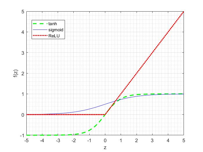
(4) $\begin{equation*} f(z)=max(0,x) \end{equation*}$

In practice, for deep Neural Networks, rectiﬁed linear function often works better than thesigmoid and the tanh functions.

The following figure shows the plots of the sigmoid, tanh and rectiﬁed linear functions (ReLU).

Neural Networks: plots of the sigmoid, tanh and rectiﬁed linear functions

Multi-Layer Neural Network

The simplest neural network described above is a very limited model. To form a multi-layer neural network, we can hook together the simple neurons. The output of a neuron can be the input of another.

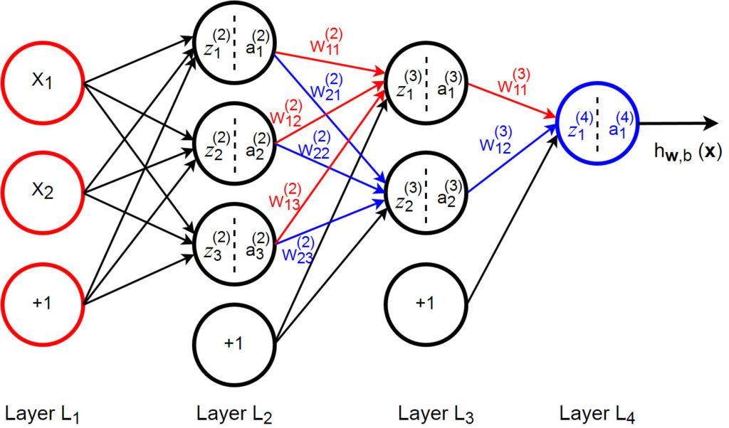
The following figure shows a simple multi-layer neural network with two hidden layers.

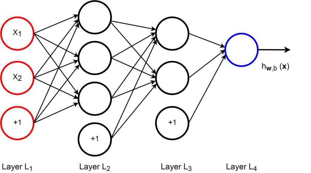
Neural Networks: a simple multi-layer neural network

This network has four layers with two inputs $x_1$ and $x_2$ in the input layer (layer $L_1$ ) and one output in the output layer (layer $L_4$ ). It has two hidden layers, layer $L_2$ and layer $L_3$ . The circles labeled “+1” are called bias units that correspond to the intercept term.

Feed Forward Propagation

Now, we’re going to analyze this multi-layer neural network.

We write $W_{ij}^{(l)}$ to denote the parameter (or weight) associated with the connection between unit $j$ in layer $l$ , and unit $i$ in layer $l+1$ . The number of layers in the network is denoted by $n_l$ . So, the above multi-layer neural network model has $n_l$ =4.

The activation of unit $i$ in layer $l$ is denoted by $a_i^ {(l)}$ . For example: for $l=1$ , we denote $a_i^{(1)}$ for activation of unit $i$ in layer 1.

We also use $a_i^{(1)}= x_i$ to denote the $i$ th input.

Given a fixed setting of the parameters $W$ and $b$ , our neural network defines a hypothesis $h_{W,b}(x)$ . It outputs a real number.

Now, we are going to look particularly at the last two layers, $L_3$ and $L_4$ .

The layer $L_4$ produces the output hypothesis and the layer $L_3$ is the last hidden layer. Specifically, the computation of the activation function in the layer $L_3$ can be derived as the following:

(5) $\begin{equation*} \begin{split} a_1^{(3)}=f(W_{11}^{(2)}a_1^{(2)}+W_{12}^{(2)}a_2^{(2)}+ W_{13}^{(2)}a_3^{(2)}+ b_1^{(2)})\\ a_2^{(3)}=f(W_{21}^{(2)}a_1^{(2)}+W_{22}^{(2)}a_2^{(2)}+ W_{23}^{(2)}a_3^{(2)}+ b_2^{(2)})\\ \end{split} \end{equation*}$

The hypothesis of the output of this neural network can be written as:

(6) $\begin{equation*} h_{wb} (x)= a_1^{(4)} =f(W_{11}^{(3)}a_1^{(3)} + W_{12}^{(3)} a_2^{(3)}) \end{equation*}$

If we let $z_{i}^{(l)}$ denoted as the total weighted sum of inputs to unit $i$ in layer $l$ , including the bias term, we will have:

(7) $\begin{equation*} \begin{split} z_i^{(l)}=\sum_{j=1}^n W_{ij}^{(l-1)}a_j^{(l-1)}+ b_i^{(l-1)}\ \end{split} \end{equation*}$

so that: $a_i^{(l)}=f(z_i^{(l)})$

or, for the computation of the next layer $l+1$ is:

(8) $\begin{equation*} \begin{split} z_i^{(l+1)}=\sum_{j=1}^n W_{ij}^{(l)}a_j^{(l)}+ b_i^{(l)}\ \end{split} \end{equation*}$

Using matrix-vectorial notation, the above equation 8 can be written as follows:

(9) $\begin{equation*} \begin{split} \textbf{z}^{(l+1)}=\textbf{W}^{(l)}\textbf{a}^{(l)}+\textbf{b}^{(l)}\ \end{split} \end{equation*}$

so that:

(10) $\begin{equation*} \begin{split} \textbf{a}^{(l+1)} & =f(\textbf{z}^{(l+1)}) \\ & =f(\textbf{W}^{(l)}\textbf{a}^{(l)}+\textbf{b}^{(l)})\\ \end{split} \end{equation*}$

The output of 6 can be written as:

(11) $\begin{equation*} \begin{split} h_{wb} (x) & = \textbf{a}^{(4)} \\ & =f(\textbf{z}^{(4)}) \\ & = f(\textbf{W}^{(3)}\textbf{a}^{(3)}+\textbf{b}^{(3)})\\ \end{split} \end{equation*}$

Back Propagation

Suppose we have a fixed training set $\lbrace (x^{(1)}, y^{(1)}),….,(x^{(m)}, y^{(m)}) \rbrace$ of $m$ training examples. We can train our neural network using batch gradient descent. For a single training example, the cost function with respect to single example is written as one-half square error as follows:

(12) $\begin{equation*} J(W,b;x,y)= \frac{1}{2} \Vert h_{W,b} (x)-y \Vert^2 \end{equation*}$

Given a training set of $m$ examples, we then define the overall cost function to be:

(13) $\begin{equation*} \begin{split} J(W,b;x,y) & = [\frac{1}{m} \sum_{i=1}^m J(W,b;x^{(i)},y^{(i)})] +\frac{\lambda}{2} \sum_{l=1}^{n_l-1} \sum_{i=1}^{s_l} \sum_{j=1}^{s_{l+1}} (W_{ji}^{(l)})^2\\ & = [\frac{1}{m} \sum_{i=1}^m ( \frac{1}{2} \Vert h_{W,b}( x^{(i)})-y^{(i)} \Vert ^2 )] +\frac{\lambda}{2} \sum_{l=1}^{n_l-1} \sum_{i=1}^{s_l} \sum_{j=1}^{s_{l+1}} (W_{ji}^{(l)})^2\\ \end{split} \end{equation*}$

The first term is an average sum-of-squares error term. The second term is a regularization term (also called a weight decay term) that tends to decrease the magnitude of the weights, and helps prevent over-fitting. The weight decay parameter $\lambda$ controls the relative importance of the two terms.

Gradient Descent

When we train the NNs, the goal is to minimize J(W,b) as a function of W and b. So basically, we initialize all parameters $W_{ij}^{(l)}$ and $b_{i}^{(l)}$ to small random values and then apply the Gradient Descent algorithm to optimize these parameters.

To implement gradient descent algorithm, the parameters of the gradient $W,b$ must be updated as follows:

(14) $\begin{equation*} \begin{split} W_{ij}^{(l)} & = W_{ij}^{(l)} - \alpha \frac{\partial}{W_{ij}^{(l)}} J(W,b)\\ b_i^{(l)} & =b_i^{(l)} -\alpha \frac{\partial}{b_i^{(l)}} J(W,b)\\ \end{split} \end{equation*}$

where $\alpha$ is the learning rate.

To do back propagation completely, the derivative of the overall cost function J(W,b) can be computed as:

(15) $\begin{equation*} \begin{split} \frac{\partial}{W_{ij}^{(l)}} J(W,b) & = \left[ \frac{1}{m} \sum_{i=1}^m \frac{\partial}{W_{ij}^{(l)}} J(W,b;x^{(i)},y^{(i)})\right] +\lambda W_{ij}^{(l)}\\ \frac{\partial}{b_i^{(l)}} J(W,b) & = \left[ \frac{1}{m} \sum_{i=1}^m \frac{\partial}{b_i^{(l)}} J(W,b;x^{(i)},y^{(i)})\right]\\ \end{split} \end{equation*}$

Detail of back propagation algorithm is:

Perform a feedforward pass, computing the activations for layers $L_2, L_3,$ and so on up to the output layer $L_{n_l}$ .
For each output unit $i$ in layer $n_l$ (the output layer), set:
(16) $\begin{equation*}\begin{split}\delta_i^{(n_l)}= \frac{\partial}{\partial z_i^{(n_l)} } \frac{1}{2} \Vert y- h_{W,b}(x) \Vert^2 =-(y_i - a_i^{(n_l)} . f'(z_i^{(n_l)})\end{split}\end{equation*}$
For $l=n_l-1,n_l-2,n_l-3, …, 2$
For each node $i$ in layer, set:
(17) $\begin{equation*}\delta_i^{(l)} = \left( \sum_{j=1}^{s_{l+1}} W_{ji}^{(l)} \delta_j^{(l+1)}\right) f'(z_i^{(l)})\end{equation*}$
Compute the desired partial derivatives, which are given as:
(18) $\begin{equation*} \begin{split} \frac{\partial}{W_{ij}^{(l)}} J(W,b;x,y) & =a_j^{(l)} \delta_i^{(l+1)}\\ \frac{\partial}{b_i^{(l)}} J(W,b;x,y) & =\delta_i^{(l+1)}\\ \end{split} \end{equation*}$

In the matrix-vectorial notation, the algorithm above can be re-written as:

Perform a feedforward pass by computing the activations for layers $L_2, L_3,$ and so on up to the output layer $L_{n_l}$ .
For output layer (layer $n_l$ ) , set:
(19) $\begin{equation*}\begin{split} \delta^{(n_l)}= -(y - a^{(n_l)} . f'(z^{(n_l)})\end{split}\end{equation*}$
For $l=n_l-1,n_l-2,n_l-3, …, 2$ , set:
(20) $\begin{equation*}\delta^{(l)} = \left( (W^{(l)})^T \delta^{(l+1)} . f'(z^{(l)}) \right) \end{equation*}$
Compute the desired partial derivatives, which are given as:
(21) $\begin{equation*} \begin{split} \nabla_{W^{(l)}} J(W,b;x,y) & =\delta^{(l+1)} (a^{(l)})^T\\ \nabla_{b^{(l)}} J(W,b;x,y) & =\delta^{(l+1)} \\ \end{split} \end{equation*}$

Now, we are ready to derive the full Gradient Descent Algorithm.

Set $\triangle W^{(l)} := \triangle b^{(l)} := 0$
For $i=1$ to $m$ ,
(a) Use back propagation to compute $\nabla_W^{(l)} J(W,b;x,y)$ and $\nabla_{b^{(l)}} J(W,b;x,y)$
(b) $\triangle W^{(l)} := \triangle W^{(l)} + \nabla_W^{(l)} J(W,b;x,y)$
(c) $\triangle b^{(l)} := \triangle b^{(l)} + \nabla_b^{(l)} J(W,b;x,y)$
Update the parameters:
(22) $\begin{equation*} \begin{split} W^{(l)} & = W^{(l)} - \alpha \left[ \left( \frac{1}{m}\triangle W^{(l)} \right) + \lambda W^{(l)} \right] \\ b^{(l)} & = b^{(l)} - \alpha \left[ \frac{1}{m}\triangle b^{(l)} \right] \\ \end{split} \end{equation*}$

Finally, the NNs now can be trained by repeating the gradient descent steps to reduce the cost function $\textbf{\textit{J}}(\textbf{\textit{W}},\textbf{\textit{b}})$ .

Reference

Andrew Ng et.al, ‘Welcome to the Deep Learning Tutorial!: Multi-Layer Neural Network’, http://deeplearning.stanford.edu/tutorial