Object Tracking: Simple Implementation of Kalman Filter in Python

Posted by Rahmad Sadli on February 15, 2020 in Object Tracking, Python Programming

Introduction

Kalman filtering is an algorithm that allows us to estimate the state of a system based on observations or measurements. It is a valuable tool for various applications, such as object tracking, autonomous navigation systems, and economic prediction.

Although the Kalman filter is a relatively simple algorithm, implementing it in a programming language like Python can be challenging for some individuals. That is why I have written this tutorial – to simplify the process and provide a clear practical approach to help you better understand the algorithm, especially for those who may find it difficult to grasp.

While many resources provide in-depth explanations of the theory behind the Kalman filter, this article focuses solely on its practical usage and does not cover the theory in depth. With a practical approach, this tutorial will help you better understand the algorithm and apply it in a real-world scenarios.

After completing this tutorial, you will have a solid foundation to effectively understand and apply the Kalman filter in tracking an object in a 1-D direction using Python. This tutorial will serve as a prerequisite for learning 2-D object tracking, which I have already covered in another post that you can find here: Object Tracking: 2-D Object Tracking using Kalman Filter in Python.

Exciting news, everyone! I’m absolutely thrilled to announce the completion of my book:

Beginner’s Guide to Multi-Object Tracking with Kalman Filter

Get 25% OFF!

Use coupon code: MIJY159IMW during checkout

Don’t miss out on the chance to become a genuine expert in this field. Grab this practical book now and embark on your journey to mastery!

Kalman Filtering Algorithm

Given the tutorial’s objective to demonstrate the practical implementation of the Kalman filter in a computer program, it is important to note that all discussions related to the filter are specific to the Discrete Kalman filter.

The basic idea of the Kalman filter is that by using the prior knowledge of the state, the filter makes a forward projection state or predicts the next state.

The Kalman Filter is intended to estimate the state of a system at time $k$ , using the linear stochastic difference equation. It assumes that the state of a system at time $k$ evolved from the prior state at time $k-1$ , expressed in the following form:

(1) $\begin{equation*}$ \textbf{x}_k=A\textbf{x}_{k-1}+B \textbf{u} _{k-1}+ \textbf{w} _{k-1}$ \end{equation*}$

It is always paired with the measurement model $\textbf{z}_k$ that describes a relation between the state and measurement at the current step $k$ . It is written as:

(2) $\begin{equation*} $ \textbf{z}_k = H \textbf{x}_k+ \textbf{v}_k$\end{equation*}$

where:

$A$ , a matrix $n x n$ , is the state transition matrix relating the previous time step ${k-1}$ to the current state $k$
$B$ , a matrix $n x l$ , is a control input matrix applied to the optional control input $\textbf{u}_{k-1}$
$H$ , a matrix $m x n$ , is a transformation matrix that transforms the state into the measurement domain
$\textbf{w}_k$ and $\textbf{v}_k$ represent the process noise vector with the covariance $Q$ and the measurement noise vector with the covariance $R$ , respectively. They are assumed statistically independence Gaussian noise with the normal probability distribution.

(3) $\begin{equation*} $p\left( w \right) \sim N(0,Q)\\$ $p\left( v \right) \sim N(0,R)$ \end{equation*}$

Kalman Equations

There are two terms used in the Kalman filter equations: a priori and a posteriori estimates. The a priori estimates represent the predicted state and error covariance based on the system dynamics and the previously estimated state. In contrast, the a posteriori estimates represent the state and error covariance after incorporating the new measurement, which are referred to as the updated state and error covariance. The following notations are used to represent these terms: $\hat{\mathbf{x}}^{-}_k$ and $\mathbf{P}^{-}_k$ denote the \textit{a priori} estimates for the state and error covariance, respectively, while $\hat{\mathbf{x}}_k$ and $\mathbf{P}_k$ denote the \textit{a posteriori} estimates for the state and error covariance, respectively.

The equations of the Kalman filter are divided into two groups: the time update equations, also referred to as the predictor equations, and the measurement update equations, which can be considered as the corrector equations. In some literature, these two terms are sometimes referred to as predictor-corrector or prediction-update.

The time update equations are responsible for projecting the current state and error covariance estimates forward to obtain the a priori estimates for the next time step. The measurement update equations are responsible for obtaining the a posteriori estimates by incorporating a new measurement into the a priori estimates.

Time Update Equations

In time update equation we’re going to calculate the predicted state estimate (a priori state estimate) $\textbf { \^{x}}^{-}_k$ and predicted error covariance (a priori error covariance estimate) $\textbf {P}^{-}_k$ .

First, the a priori state estimate $\textbf { \^{x}}^{-}_k$ is predicted by using the state dynamic equation model that projects forward one step in time as follows:

(4) $\begin{equation*}$ \textbf { \^{x}}^{-}_k = A \textbf{\^{x}}_{k-1}+B \textbf{u} _{k-1}$ \end{equation*}$

where: $\textbf{\^{x}}_{k-1}$ is the previous estimated state (a posteriori state estimate).

Next, the error covariance matrix $\textbf {P}^{-}_k$ is predicted by:

(5) $\begin{equation*}$ \textbf {P}^{-}_k = A \textbf{P}_{k-1}A^T+ \textbf{Q} $ \end{equation*}$

where $\textbf{P}_{k-1}$ is the previous estimated error covariance matrix and $\textbf{Q}$ is the process noise covariance.

Measurement Update Equations

During the update stage, we compute the Kalman gain $\textbf {K}_k$ as follows:

(6) $\begin{equation*}$ \textbf {K}_k = \textbf{P}^{-}_kH^T$(H\textbf{P}^{-}_kH^T+ \textbf{R} )^{-1}$ \end{equation*}$

where $\textbf{R}$ is the measurement noise covariance.

After that, we perform the actual measurement $\textbf {z}_k$ .

In order to update the predicted state estimate $\textbf { \^{x}}^{-}_k$ , we need to measure the measurement residual. It is the difference between the true measurement $\textbf {z}_k$ and the predicted measurement $H\textbf{\^{x}} ^{-}_k$ . So the measurement residual is $\textbf {z}_k - H\textbf{\^{x}} ^{-}_k$ .

To update the predicted state estimate called updated state estimed $\textbf {\^{x}}_k$ is proceed by performing the summation of the a priori projected state estimate $\textbf { \^{x}}^{-}_k$ to the product of the Kalman gain and the measurement residual. It can be written as follows:

(7) $\begin{equation*}$ \textbf {\^{x}}_k = \textbf{\^{x}}^{-}_k+ \textbf{K}_k(\textbf{z}_k-H \textbf{\^{x}} ^{-}_k)$ \end{equation*}$

After obtaining the updated state estimate, the filter calculates the updated error covariance ( a posteriori error covariance estimate) $\textbf{P}_k$ , which will be used in the next time step.

(8) $\begin{equation*} $\textbf{P}_k = (I - \textbf{K}_kH) \textbf{P}^{-}_k$\end{equation*}$

where $I$ is an identity matrix.

The following tables 1 and 2 show the summary of the Kalman filter algorithm.

Tabel 1. Discrete Kalman Time update equations

=======================================

(9) $\begin{equation*}$ \textbf { \^{x}}^{-}_k = A \textbf{\^{x}}_{k-1}+B \textbf{u} _{k-1}$ \end{equation*}$

(10) $\begin{equation*}$ \textbf {P}^{-}_k = A \textbf{P}_{k-1}A^T+ \textbf{Q} $ \end{equation*}$

=======================================

Tabel 2. Discrete Kalman filter measurement update equations.

========================================================

(11) $\begin{equation*}$ \textbf {K}_k = \textbf{P}^{-}_kH^T$(H\textbf{P}^{-}_kH^T+ \textbf{R} )^{-1}$ \end{equation*}$

(12) $\begin{equation*}$ \textbf {\^{x}}_k = \textbf{\^{x}}^{-}_k+ \textbf{K}_k(\textbf{z}_k-H \textbf{\^{x}} ^{-}_k)$ \end{equation*}$

(13) $\begin{equation*} $\textbf{P}_k = (I - \textbf{K}_kH) \textbf{P}^{-}_k$ \end{equation*}$

========================================================

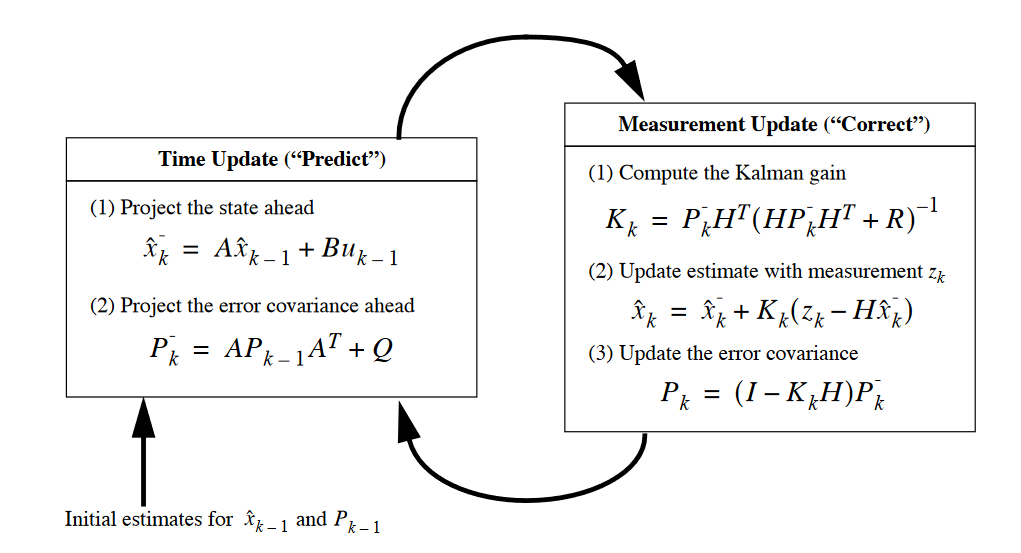
The figure below descibes the cycle of ongoing discrete Kalman filter.

Initially, to implement the Kalman filter we need to guess an initial state $\textbf{\^{x}}_{k-1}$ and error covariance matrix $\textbf{P}_{k-1}$ . The current state estimate will be projected forward to obtain the a priori estimates for the next time step by the time update equations. Then, using the actual measurement, the measurement update equations adjust the projected estimate at that time.

That’s it for Kalman filter theory…

Next…

We’re going to look at a simple one-dimensional object tracking problem.

Implementation

In this example, we want to model a moving object following a simple track as given in the following function:

(14) $\begin{equation*}f(t)=0.1*(t^2-t)\end{equation*}$

Our task is to track that object using the Kalman filter from time $t$ =0 to $t$ =100 $s$ .

So, let’s get started..

State transition matrix A and control matrix B

Based on Kinematic equation, the relation between the position $x$ and velocity $\dot x$ can be written as the following:

Position:

(15) $\begin{equation*}x_{k} =x_{k-1}+ \dot x_{k-1}\Delta t+ \frac{1}{2} \ddot x_{k-1}(\Delta{t})^2}\\\end{equation*}$

Velocity:

(16) $\begin{equation*} \dot x_{k} = \dot x_{k-1}+ \ddot x_{k-1}\Delta{t} \end{equation*}$

where: $\ddot x$ is the acceleration.

Since the state vector $\textbf{x}_k$ contains the position and velocity, we can model this example as follows:

(17) $\begin{equation*}\textbf{x}_k = \begin{bmatrix} x_k\\ \dot x_k \\ \end{bmatrix} = \begin{bmatrix} x_{k-1}+ \dot x_{k-1}\Delta t+ 1/2 \ddot x_{k-1}\Delta{t^2}}\\ \dot x_{k-1}+ \ddot x_{k-1}\Delta{t} \\ \end{bmatrix} \end{equation*}$

These linear equations can be written in matrix form as:

(18) $\begin{equation*}\textbf{x}_k = \begin{bmatrix}x_k\\ \dot x_k \\ \end{bmatrix} = \begin{bmatrix} 1 & \Delta{t}\\0 & 1\\ \end{bmatrix} \begin{bmatrix} x_{k-1} \\ \dot x_{k-1} \\ \end{bmatrix} + \begin{bmatrix} \frac{1}{2}(\Delta{t})^2 \\ (\Delta{t} \\ \end{bmatrix} \ddot x_{k-1} \end{equation*}$

The equation (18) can be written as:

(19) $\begin{equation*}\textbf{x}_k = \begin{bmatrix} 1 & \Delta{t}\\0 & 1\\ \end{bmatrix} \textbf{x}_{k-1} + \begin{bmatrix} \frac{1}{2}(\Delta{t})^2 \\ \Delta{t} \\ \end{bmatrix} \ddot x_{k-1} \end{equation*}$

By comparing the eq.(19) to the eq.(1), we have the following relations:

(20) $\begin{equation*} \textbf{A} = \begin{bmatrix} 1 & \Delta{t}\\0 & 1\\ \end{bmatrix} \end{equation*}$

and

(21) $\begin{equation*} \textbf{B} = \begin{bmatrix} \frac{1}{2}(\Delta{t})^2 \\ \Delta{t} \\ \end{bmatrix} \end{equation*}$

Transformation matrix H

Measurements of the system can be performed according to the model in eq.(2):

(22) $\begin{equation*} $ \textbf{z}_k = H \textbf{x}_k+ \textbf{v}_k$\end{equation*}$

Since we only measure the position, the eq.(22) can be written in matrix form as:

(23) $\begin{equation*}\textbf{z}_k = \begin{bmatrix} 1 & 0\end{bmatrix} \begin{bmatrix} x_k \\ \dot x_k \\ \end{bmatrix} + \textbf{v}_{k} \end{equation*}$

So, we have the transformation matrix $H$ as follows:

(24) $\begin{equation*} \textbf{H}= \begin{bmatrix} 1 & 0\end{bmatrix} \end{equation*}$

Process noise covariance matrix Q

The process noise covariance matrix $\textbf{Q}$ or error in the state process is basically can be written as follows:

(25) $\begin{equation*} \textbf{Q} = \begin{bmatrix} \sigma^2_x & \sigma_x \sigma_{\dot x} \\ \sigma_{\dot x} \sigma_x & \sigma^2_ {\dot x} \\ \end{bmatrix} \end{equation*}$

where $\sigma_x$ and $\sigma_{\dot x}$ are the standard deviations of the position and the velocity, respectively.

We can define the standard deviation of position as the standard deviation of acceleration $\sigma_a$ multiplied by $\frac{\Delta{t^2}}{2}$ . The reason for this is because the $\frac{\Delta{t^2}}{2}$ is the effect that will have on the position. Therefore, by multiplying the standard deviation of the acceleration by $\frac{\Delta{t^2}}{2}$ we’ll have the standard deviation of the position.

Similarly, if we multiply the standard deviation of the acceleration by delta $\Delta{t}$ , we’ll get the standard deviation of the velocity.

So, we can write the process covariance noise $\textbf{Q}$ as follows:

(26) $\begin{equation*} \textbf{Q} = \begin{bmatrix} \frac{\Delta{t^4}}{4} & \frac{\Delta{t^3}}{2} \\ \frac{\Delta{t^3}}{2} & \Delta{t^2} \\ \end{bmatrix} \sigma^2_a \end{equation*}$

where \sigma_a is the tuning magnitude of standard deviation of the acceleration.

Measurement noise covariance matrix R

The covariance of the measurement noise $R$ is a scalar and is equal to the variance of the measurement noise. It can be written as:

(27) $\begin{equation*} R=\sigma^2_z \end{equation*}$

Now we’re ready to implement it in Python.

Python Implementation

In this example, we assume that the standard deviations of the acceleration $\sigma_a$ and the measurement $\sigma_z$ are 0.25 $m/s^2$ and 1.2 $m$ , respectively. Then, we suppose also that the acceleration magnitude $a$ is 2.0 $m/s$ . The position will be estimated every 0.1 $s$ .

Now, we’re ready to write our Kalman filter code. First, we create a class called KalmanFilter. We initialize the class with four parameters, they are dt (time for 1 cycle), u (control input related to the acceleration), std_acc (standard deviation of the acceleration, $\sigma_a$ ), and std_meas (standard deviation of the measurement, $\sigma_z$ ).

class KalmanFilter(object):
    def __init__(self, dt, u, std_acc, std_meas):
        self.dt = dt
        self.u = u
        self.std_acc = std_acc
        self.A = np.matrix([[1, self.dt],
                            [0, 1]])
        self.B = np.matrix([[(self.dt**2)/2], [self.dt]]) 
        self.H = np.matrix([[1,0]])
        self.Q = np.matrix([[(self.dt**4)/4, (self.dt**3)/2],
                            [(self.dt**3)/2, self.dt**2]]) * self.std_acc**2
        self.R = std_meas**2
        self.P = np.eye(self.A.shape[1])
        self.x = np.matrix([[0],[0]])

Then create a function predict() that contains time update equations, eq.(4) and eq.(5) as follows:

    def predict(self):
        # Ref :Eq.(9) and Eq.(10)

        # Update time state
        self.x = np.dot(self.A, self.x) + np.dot(self.B, self.u)

        # Calculate error covariance
        # P= A*P*A' + Q
        self.P = np.dot(np.dot(self.A, self.P), self.A.T) + self.Q
        return self.x

Then we create a function update() that contains measurement update equations, eq.(11), eq.(12) and eq.(13) as follows:

    def update(self, z):
        # Ref :Eq.(11) , Eq.(11) and Eq.(13)
        # S = H*P*H'+R
        S = np.dot(self.H, np.dot(self.P, self.H.T)) + self.R

        # Calculate the Kalman Gain
        # K = P * H'* inv(H*P*H'+R)
        K = np.dot(np.dot(self.P, self.H.T), np.linalg.inv(S))  # Eq.(11)

        self.x = np.round(self.x + np.dot(K, (z - np.dot(self.H, self.x))))  # Eq.(12)

        I = np.eye(self.H.shape[1])
        self.P = (I - (K * self.H)) * self.P  # Eq.(13)

And, here is our main() function:

def main():
    dt = 0.1
    t = np.arange(0, 100, dt)

    # Define a model track
    real_track = 0.1*((t**2) - t)

    u= 2
    std_acc = 0.25     # we assume that the standard deviation of the acceleration is 0.25 (m/s^2)
    std_meas = 1.2    # and standard deviation of the measurement is 1.2 (m)

    # create KalmanFilter object
    kf = KalmanFilter(dt, u, std_acc, std_meas)

    predictions = []
    measurements = []
    for x in real_track:
        # Mesurement
        z = kf.H * x + np.random.normal(0, 50)

        measurements.append(z.item(0))
        predictions.append(kf.predict()[0])
        kf.update(z.item(0))


    fig = plt.figure()

    fig.suptitle('Example of Kalman filter for tracking a moving object in 1-D', fontsize=20)

    plt.plot(t, measurements, label='Measurements', color='b',linewidth=0.5)

    plt.plot(t, np.array(real_track), label='Real Track', color='y', linewidth=1.5)
    plt.plot(t, np.squeeze(predictions), label='Kalman Filter Prediction', color='r', linewidth=1.5)

    plt.xlabel('Time (s)', fontsize=20)
    plt.ylabel('Position (m)', fontsize=20)
    plt.legend()
    plt.show()

if __name__ == '__main__':
    main()

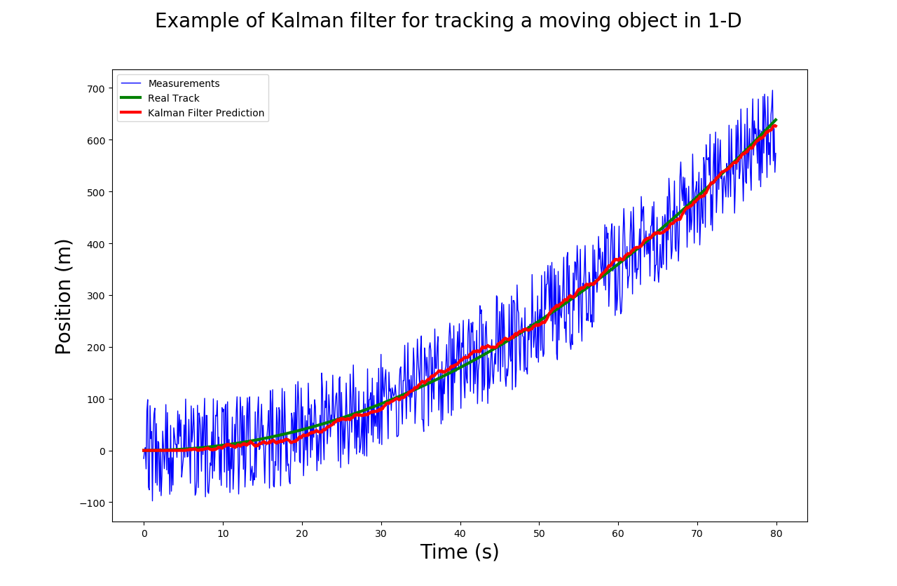
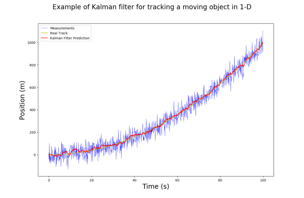
The following figure shows the simulation performance of 1-D Kalman Filter for the above case. We can see that it works pretty well.

The code of this implementation can be also found in my Github repo in this link.

Link to 2-D Object Tracking:

Object Tracking: 2-D Object Tracking using Kalman Filter in Python

Here are the related posts in the Python category that you might want to take a look:

Reference

What others say

Object Tracking: 2-D Object Tracking using Kalman Filter in Python - says:

February 26, 2020 at 12:41 pm

[…] using the same philosophy as what we’ve discussed earlier in my previous tutorial for 1-D Kalman Filter, we can rewrite the process noise covariance matrix for 2-D Kalman Filter […]

Reply
Rian says:

February 26, 2020 at 2:50 pm

very helpful

Reply
Ryan says:

February 26, 2020 at 3:23 pm

suitable for study

Reply
- rahmadsadli says:
  
  February 27, 2020 at 9:10 pm
  
  Thank you. I hope this will be useful.
  
  Reply
Manish Kumar says:

March 11, 2020 at 9:47 am

Thank you Very Much its very helpful

Reply
- rahmadsadli says:
  
  April 19, 2020 at 7:07 pm
  
  Hi, you’re welcome.
  
  Reply
- rahmadsadli says:
  
  March 11, 2020 at 5:52 pm
  
  You’re welcome, I’m glad it helps.
  
  Reply
JayMnM says:

June 1, 2020 at 4:21 am

cool…thanks a lot!!

Reply
newbie says:

February 16, 2021 at 11:59 am

Firstly, thanks a lot for your contribution. I wonder what differs in code when I use an already gathered dataset containing time-altitude data and try to apply KalmanFilter in it. I have no acceleration or any other data. would be more than happy if you can help. (urgent!)

Reply
david thompsons says:

January 7, 2022 at 3:13 am

What’s with the “np.round” on line 10 of update. My expected acceleration was very small (absolute value) and this almost made me believe something serious was wrong with how I was running my data with this filter.

Reply
canadian pharcharmy says:

October 18, 2023 at 5:17 pm

Wonderful, what a blog it is! This blog gives helpful information to us, keep it up.

Reply